Memory Scaling on Haswell CPU, IGP and dGPU: DDR3-1333 to DDR3-3000 Tested with G.Skill
by Ian Cutress on September 26, 2013 4:00 PM ESTOne side I like to exploit on CPUs is the ability to compute and whether a variety of mathematical loads can stress the system in a way that real-world usage might not. For these benchmarks we are ones developed for testing MP servers and workstation systems back in early 2013, such as grid solvers and Brownian motion code. Please head over to the first of such reviews where the mathematics and small snippets of code are available.
3D Movement Algorithm Test
The algorithms in 3DPM employ uniform random number generation or normal distribution random number generation, and vary in various amounts of trigonometric operations, conditional statements, generation and rejection, fused operations, etc. The benchmark runs through six algorithms for a specified number of particles and steps, and calculates the speed of each algorithm, then sums them all for a final score. This is an example of a real world situation that a computational scientist may find themselves in, rather than a pure synthetic benchmark. The benchmark is also parallel between particles simulated, and we test the single thread performance as well as the multi-threaded performance. Results are expressed in millions of particles moved per second, and a higher number is better.
Single threaded results:
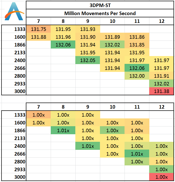
For software that deals with a particle movement at once then discards it, there are very few memory accesses that go beyond the caches into the main DRAM. As a result, we see little differentiation between the memory kits, except perhaps a loose automatic setting with 3000 C12 causing a small decline.
Multi-Threaded:
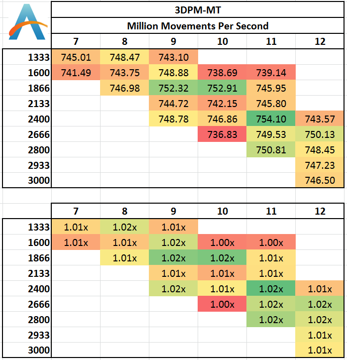
With all the cores loaded, the caches should be more stressed with data to hold, although in the 3DPM-MT test we see less than a 2% difference in the results and no correlation that would suggest a direction of consistent increase.
N-Body Simulation
When a series of heavy mass elements are in space, they interact with each other through the force of gravity. Thus when a star cluster forms, the interaction of every large mass with every other large mass defines the speed at which these elements approach each other. When dealing with millions and billions of stars on such a large scale, the movement of each of these stars can be simulated through the physical theorems that describe the interactions. The benchmark detects whether the processor is SSE2 or SSE4 capable, and implements the relative code. We run a simulation of 10240 particles of equal mass - the output for this code is in terms of GFLOPs, and the result recorded was the peak GFLOPs value.
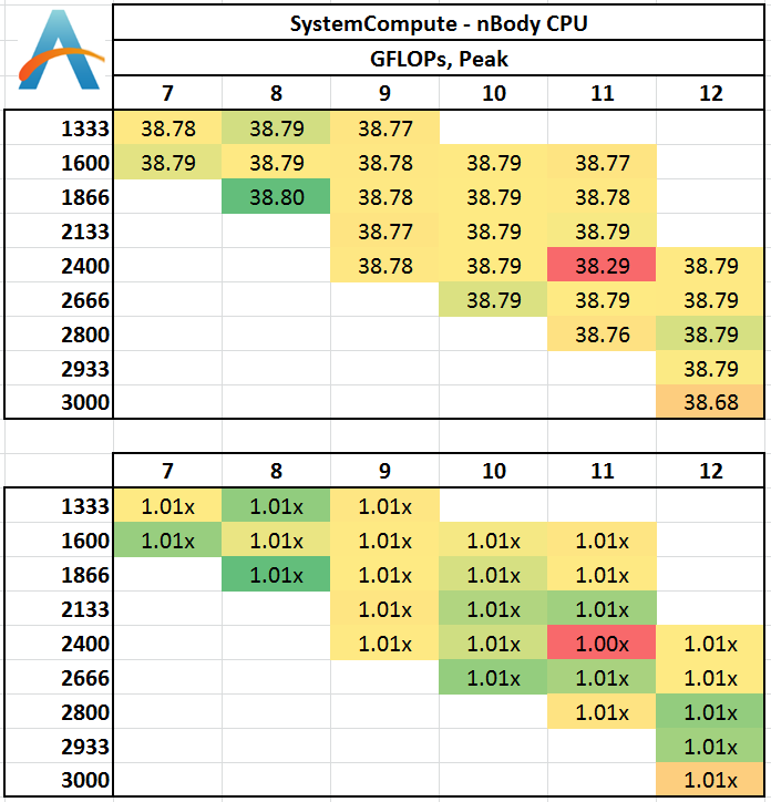
Despite co-interaction of many particles, the fact that a simulation of this scale can hold them all in caches between time steps means that memory has no effect on the simulation.
Grid Solvers - Explicit Finite Difference
For any grid of regular nodes, the simplest way to calculate the next time step is to use the values of those around it. This makes for easy mathematics and parallel simulation, as each node calculated is only dependent on the previous time step, not the nodes around it on the current calculated time step. By choosing a regular grid, we reduce the levels of memory access required for irregular grids. We test both 2D and 3D explicit finite difference simulations with 2n nodes in each dimension, using OpenMP as the threading operator in single precision. The grid is isotropic and the boundary conditions are sinks. We iterate through a series of grid sizes, and results are shown in terms of ‘million nodes per second’ where the peak value is given in the results – higher is better.
Two-Dimensional Grid:
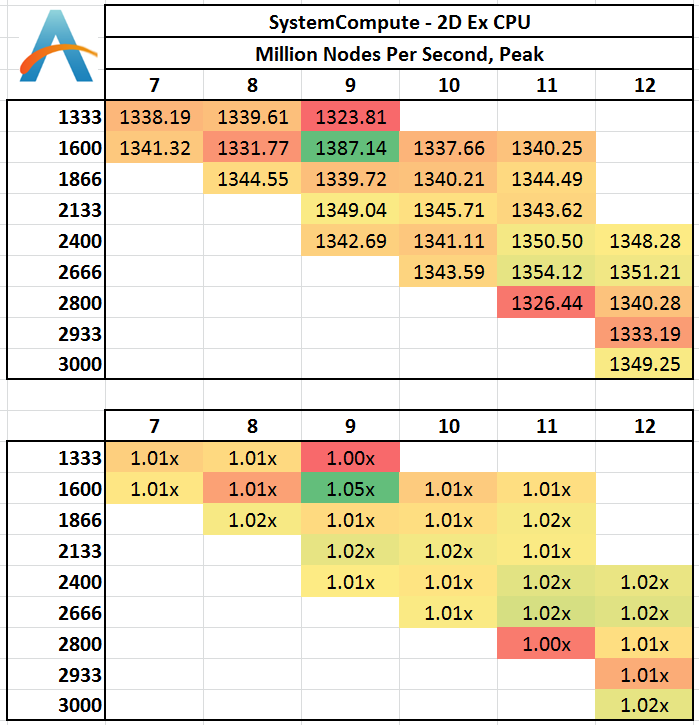
In 2D we get a small bump over at 1600 C9 in terms of calculation speed, with all other results being fairly equal. This would statistically be an outlier, although the result seemed repeatable.
Three Dimensions:
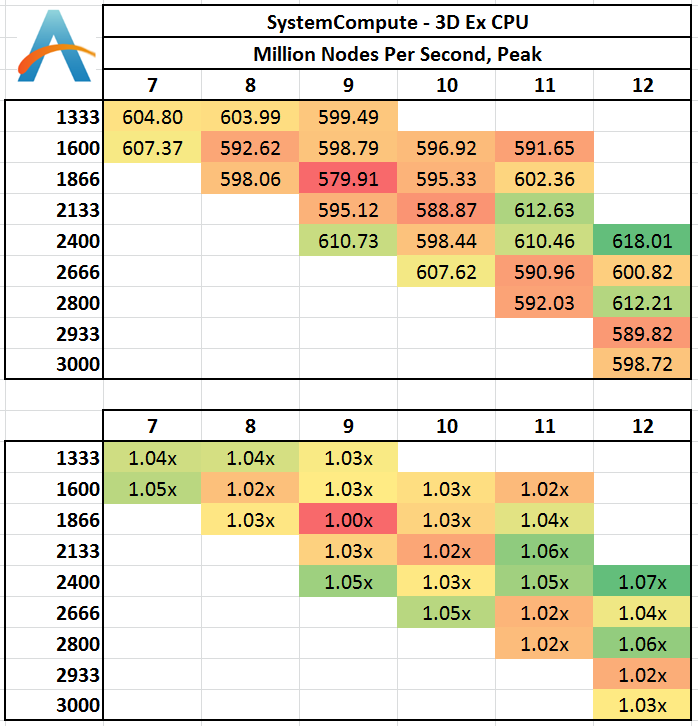
In three dimensions, the memory jumps required to access new rows of the simulation are far greater, resulting in L3 cache misses and accesses into main memory when the simulation is large enough. At this boundary it seems that low CAS latencies work well, as do memory speeds > 2400 MHz. 2400 C12 seems a surprising result.
Grid Solvers - Implicit Finite Difference + Alternating Direction Implicit Method
The implicit method takes a different approach to the explicit method – instead of considering one unknown in the new time step to be calculated from known elements in the previous time step, we consider that an old point can influence several new points by way of simultaneous equations. This adds to the complexity of the simulation – the grid of nodes is solved as a series of rows and columns rather than points, reducing the parallel nature of the simulation by a dimension and drastically increasing the memory requirements of each thread. The upside, as noted above, is the less stringent stability rules related to time steps and grid spacing. For this we simulate a 2D grid of 2n nodes in each dimension, using OpenMP in single precision. Again our grid is isotropic with the boundaries acting as sinks. We iterate through a series of grid sizes, and results are shown in terms of ‘million nodes per second’ where the peak value is given in the results – higher is better.
2D Implicit:
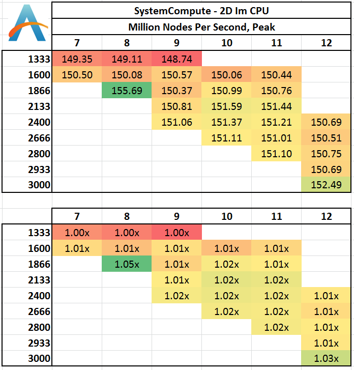
Despite the nature if implicit calculations, it would seem that as long as 1333 MHz is avoided, results are fairly similar. 1866 C8 being a surprise outlier.


89 Comments
View All Comments
ShieTar - Friday, September 27, 2013 - link
I think you would have to propose a software benchmark which benefits from actually running from a Ramdisk. Testing the RD itself with some kind of synthetic HD-Benchmark will not give you much different results than a synthetic memory benchmark, unless the software implementation is rubbish.So if you want to see this happen, I suggest you explain to everybody what kind of software you use in combination with your Ramdisk, and why it benefits from it. And hope that this software is sufficiently relevant to get a large number of people interested in this kind of benchmark.
ShieTar - Friday, September 27, 2013 - link
Two comments on the "Performance Index" used in this article:1. It is calculated as the reverse of the actual access latency (in nanoseconds). Using the reverse of a physically meaningful number will always make the relationship exhibit much more of an "diminishing return" then when using the phyical attribute directly.
2. As no algorithm should care directly about the latency, but rather about the combined time to get the full data set it requested, it would be interesting to understand which is the typical size of a data set affecting the benchmarks indicate. If your software is randomly picking single bytes from the memory, you expect performance to only depend on the latency. On the other hand, if the software is reading complete rows (512 bytes), the bandwidth becomes more relevant than the latency.
Of course figuring out the best performance metric for any kind of review can take a lot of time and effort. But when you do a review generating this large amount of data anyways, would it be possible to make the raw data available to the readers, so they can try to get their own understanding on the matter?
Death666Angel - Friday, September 27, 2013 - link
First of all, great article and really good chart layout, very easy to read! :DBut one thing seems strange, the WinRAR 3.93 test, 2800MHz/C12 performs better than 2800MHz/C11, but you call out ...C11 in the text as performing well, even though anyone can increase their latencies without incurring stability issues (that's my experience at least). Switched numbers? :)
willis936 - Friday, September 27, 2013 - link
I too thought this was strange. You could see higher latencies clock for clock performing better which doesn't seem intuitive. I couldn't work out why those results were the way they were.ShieTar - Friday, September 27, 2013 - link
In reality, there really should be no reason why a longer latency should increase performance (unless you are programming some real-time code which depends on algorithm synchronization). Therefore it seems safe to interpret the difference as the measurement noise of this specific benchmark.Urbanos - Friday, September 27, 2013 - link
excellent article! i was waiting for one of these! great work, masterful :)jaydee - Friday, September 27, 2013 - link
Great work, I'd like to see a future article look at single-channel vs dual channel RAM in laptops/mITX/NUC configurations. With only two SO-DIMM slots, people have to really evaluate whether or not you want to fill both DIMM slots knowing you'd have to replace both of them if you want to upgrade but able to utilize the dual channels, or going with a single SO-DIMM, losing the dual channel but having an easier memory upgrade path down the road.Thanks and great work!
Hrel - Friday, September 27, 2013 - link
How do you get such nice screenshots of the BIOS? They look much nicer than when people just use a camera so what did you use to take those screenshots?merikafyeah - Friday, September 27, 2013 - link
Probably used a video capture card. These are also used to objectively evaluate GPU frame-pacing in a way that software like FRAPS cannot.Rob94hawk - Saturday, September 28, 2013 - link
Moder BIOS allow you to upload screenshots to USB. My MSI Z87 Gaming does it. No more picture taking. It's a great feature long overdue!