Westmere-EP to Sandy Bridge-EP: The Scientist Potential Upgrade
by Ian Cutress on March 4, 2013 9:30 AM EST- Posted in
- CPUs
- Xeon
- Westmere-EP
- Sandy Bridge-EP
Grid Solvers
For any theoretical evaluation of physical events, we mathematically track a volume and monitor the evolution of the properties within that volume (speed, temperature, concentration). How a property changes over time is defined by the equations of the system, often describing the rate of change of energy transfer, motion, or another property over time.
The volume itself is divided into smaller sections or ‘nodes’, which contain the values of the properties of the system at that point. The volume can be split a variety of different ways – regularly by squares (finite difference), irregularly by squares (finite difference with variable distance modifiers), irregularly by triangles (finite element) to name three, although many different methods exist. More often than not the system has a point of action where stuff is happening (heat transfer at a surface or a surface bound reaction), meaning that some areas of the system are more important than others and the grid solver should focus on those areas (benefits against regular finite difference). This usually comes at the expense of increased computational difficulty and irregular memory accesses, but affords faster simulation time having to calculate 1000 variable distance points rather than 1 million (as an example of a 106 simulation volume). Another point to note is that if the system is symmetrical about an axis (or the center), the simulation and grid chosen is often reduced by a dimension to improve simulation throughput (as O(n) < O(n2) < O(n3)).
Boundary conditions can also affect the simulation – because the volume being simulated is finite with edges, the action at those edges has to be determined. The volume may be one unit of a whole, making the boundary a repeating boundary (entering one side comes out the other), a reflecting boundary (rate of change at the boundary is zero), a sink (boundary is constantly 0), an input (boundary is constantly 1) or a reactive zone (rate of change is defined by kinetics or another property) – again, there are many more boundary conditions depending on the simulation at hand. However as the boundary conditions have to be treated differently, this can cause extended memory reads, additional calculations at various points, or fewer calculations by virtue of constant values.
A final point to make is dealing with simulations involving time. For the scenarios I simulated in research, time could either be dealt with as a pushing structure (every node in the next time step is based on the surrounding nodes ‘pushing‘ the values of the previous time step) or pulling structure (each calculation of the next time step requires pulling a matrix of values from the previous time step), also known as explicit and implicit respectively. By their nature, explicit simulations are embarrassingly parallel but have restricted conditions based on time step and node size – implicit simulations are only slightly parallel, require larger memory jumps but have several fewer restrictions that allow more to be simulated in less time. Deciding between these two methods is often one of the first decisions when it comes to the sorts of simulation I will be testing.
All of the simulations used in this article were described in our previous GA-7PESH1 review in terms of both mathematics and code. For the sake of brevity, please refer back to that article for more information.
Explicit Finite Difference
For any grid of regular nodes, the simplest way to calculate the next time step is to use the values of those around it. This makes for easy mathematics and parallel simulation, as each node calculated is only dependent on the previous time step, not the nodes around it on the current calculated time step. By choosing a regular grid, we reduce the levels of memory access required for irregular grids. We test both 2D and 3D explicit finite difference simulations with 2n nodes in each dimension, using OpenMP as the threading operator in single precision. The grid is isotropic and the boundary conditions are sinks.
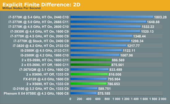
The 6-core X5690s in this situation definitely perform lower than the 8-core E5-2690s, although with the X5690s it pays to have HyperThreading turned off or face 3.5% less performance. Compared to the E5-2690s, the X5690s only perform 8% down for that 25% price difference.
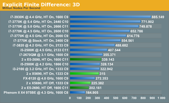
In three dimensions, the E5-2690s still have the advantage, at 7.7% with HT enabled. With HT disabled, the dual X5690 system performs 11.4% better than the Sandy Bridge-E counterparts. The nature of the 3D simulation tends towards a single CPU system performing much better, however.
Implicit Finite Difference (with the Alternating Direction Implicit method)
The implicit method takes a different approach to the explicit method – instead of considering one unknown in the new time step to be calculated from known elements in the previous time step, we consider that an old point can influence several new points by way of simultaneous equations. This adds to the complexity of the simulation – the grid of nodes is solved as a series of rows and columns rather than points, reducing the parallel nature of the simulation by a dimension and drastically increasing the memory requirements of each thread. The upside, as noted above, is the less stringent stability rules related to time steps and grid spacing. For this we simulate a 2D grid of 2n nodes in each dimension, using OpenMP in single precision. Again our grid is isotropic with the boundaries acting as sinks.
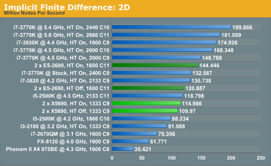
The IPC and increased memory bandwidth of the E5-2690 system comes through here, with the X5690s being 20% slower. The dual CPU nature of the system is still at odds with the coding, as a single i7-3930K at stock should perform similarly.


44 Comments
View All Comments
alpha754293 - Tuesday, March 5, 2013 - link
Sorry, I'm back. Where was I? oh yes...Unless that you were purely running single-threaded, single process jobs (or maybe even lightly multithreaded, single process jobs) - I would think that to say that it is favouring a single-CPU system might be a little bit misleading.
Even with single-socket systems, if it's got multiple cores, then you can parallelize amongst those as well.
Some commercial programs too favour 2^n cores as well, which would make quite a difference between having 8- or 16-cores vs. 6 or 12 (because some programs won't even run properly if it isn't 2^n).
Also it was interesting to see that you didn't run the implicit 3D grid solver benchmark.
Actually, MPI might not has as much to do with memory than you might think. Considering that the world's top supercomputers haven't maxed out the memory capacity per socket, I doubt that. It IS, however, much better at the actual parallelization of the task than OpenMP.
"‘Is moving from Westmere-EP to Sandy Bridge-EP a reasonable upgrade’, in the majority of our scenarios it probably is not"
It really depends. If you're writing your own code (which is what you're doing), and you have a lot of control over it, then that MIGHT be a true statement. (And it also depends on the state of your code too. If you're almost always in a permanent alpha phase (because you keep adding new capability and modules to it), then chances are, you might not even get around to parallelizing it (because you want to make sure that the base solver is robust first before you add the additional complexity of parallelization on top of that).
But if, say, suppose that you're doing research on crash and crash safety; and you're using a commercial code - some of those would just favour more cores period (see Johan's latest benchmark on the Opteron for details).
And as to whether or not you can run it on a GPU; the problem with that is that you have to make sure that every system in your working/research group has the same capable GPU hardware; otherwise, those that don't can't even run it, and those that have lesser-capable GPUs - might not get the benefits of using a GPU as much as you think, if at all.
(My GTX 660 OC's double precision performance is actually slightly SLOWER than the double precision performance of my 3930K OC'd to 4.5 GHz.)
alpha754293 - Tuesday, March 5, 2013 - link
Also, as far as I know/can remember - not everything can make use of AVX - both in terms of programs and also in terms of fundamental math operations.And I would suspect that you might also have slight performance variations if you were to recompile on the Sandy Bridge vs. on the Westmere-EP platforms (rather than sharing the binaries between the two - unless you purposely don't make it target specific).
wingless - Monday, March 4, 2013 - link
Somebody on my folding team is building this setup with dual Titans as a folding/gaming rig. The ultimate in computation, gaming, and space heating!yougotkicked - Monday, March 4, 2013 - link
I just wanted to say I found this analysis rather interesting. I'm a undergrad CS major, but I work in the IT office for the chemical engineering and material science dept. at a research university, so this breakdown of the relationship between simulations and hardware was really fascinating for me.Just to give some perspective on the pricing of an OEM-built system using E5-26XX parts, one of the research groups I work with recently bought a dual E5-2687W system from HP with 128 gigs of ram, liquid cooling, and a mid-range workstation GPU; The whole system came in at over $10,000. admittedly this includes a ~$1000 monitor and 4 hard drives, but this is probably at least a 30% margin over the cost of hardware, so the 10% margin used in the article may be on the conservative side.
P.S. we didn't suggest that system to the researchers, they bought it on their own.
colonelpepper - Monday, March 4, 2013 - link
HP & Dell systems are much more expensive than the same system built by a "system integrator" <-- I believe that's what they're calledI've read in other forums that system integrators building you a custom system add about 10% to the price tag.
yougotkicked - Monday, March 4, 2013 - link
That sounds reasonable, my only gripe would be that many researchers would not seek out a system integrator and just turn to a big name like HP. Had they sought the advice of the IT office I would have suggested we build it in-house for no markup at all.Kevin G - Monday, March 4, 2013 - link
Dell and HP's workstation lines carry a much higher premium than what you'd get DIY. The difference is in their warranties. Since dual socket workstations are effectively using low end servers in a tower chassis and they'll offer warranties very similar to what you can get for a 24/7/365 running server. While I'm not a big fan of Dell's hardware, I will say that they do follow through on their warranties. I've seen them get a replacement hard drive to my facility in under 4 hours as that is the level of support I was paying for. It wasn't cheap but it was worth it considering the business need.With the scientific slant, such warranties may turn out to be overkill as is going with OEM's. You'd still want to have the necessary data protections in place like ECC memory, redundant storage and a good backup policy while the simulation is running. However, what is the worst case that could happen when something does go wrong with the basic protections in place? Generally it is simply running the simulation again. Time is money and there are often some deadlines to meet. So if the simulation can't realistically be run again or it'd cost to much to run again, then going with an OEM that'll help achieve greater uptime is worth it.
As for the price of some of these components individually, I'm about to drop ~$1000 USD on a 128 GB memory upgrade. OEM's like Dell and HP get such parts far cheaper than DIY users due to bulk purchasing power. It is far higher than 10% margin for them in terms of raw hardware costs.
IanCutress - Tuesday, March 5, 2013 - link
The dual E5520 systems from Dell (with 4GB RAM because research department limited us to XP 32-bit) I used for research, with basic storage and a monitor each, ran up to £2k per order back in 2009. After a month of waiting to be delivered (after tons of initial hassle with the department IT guy), it turns out the systems arrived shortly after ordering and our IT guy had decided to hide them in a different building on campus and 'forgot to tell us'. The monitors were in a building the other side of campus. Fun fun fun! Needless to say, we were all rather annoyed. But looking back, I should have just asked for a single powerful Xeon workstation.yougotkicked - Tuesday, March 5, 2013 - link
Yikes, sounds like your IT guy needs to get his act together. We'd never get away with that kind of stuff here.My university has a few super-computing clusters available for researchers running truly large simulations, but because of that many groups choose not to buy systems powerful enough to run their mid-sized simulations and the clusters are usually booked a while in advance. The HP system was purchased primarily because the group was sick of waiting for their simulations to get a turn on the supercomputers.
If only there were a folding@home style client that researchers could easily program for, we could turn our computer labs into compute clusters at night.
colonelpepper - Monday, March 4, 2013 - link
This would be a very poor time to spend thousands of dollars on a high-end 2600 CPUs!The Xeon 2600 series is getting a refresh soon, better to wait and get more CPU for your buck... unless you're dying to spend big $$ now that is:
http://2.bp.blogspot.com/-zhrS1C8wbk0/UHj_HxsrMTI/...
that link is to the largest image I could find of Intel's Xeon Roadmap that was leaked late last year