Memory Scaling on Haswell CPU, IGP and dGPU: DDR3-1333 to DDR3-3000 Tested with G.Skill
by Ian Cutress on September 26, 2013 4:00 PM ESTOne side I like to exploit on CPUs is the ability to compute and whether a variety of mathematical loads can stress the system in a way that real-world usage might not. For these benchmarks we are ones developed for testing MP servers and workstation systems back in early 2013, such as grid solvers and Brownian motion code. Please head over to the first of such reviews where the mathematics and small snippets of code are available.
3D Movement Algorithm Test
The algorithms in 3DPM employ uniform random number generation or normal distribution random number generation, and vary in various amounts of trigonometric operations, conditional statements, generation and rejection, fused operations, etc. The benchmark runs through six algorithms for a specified number of particles and steps, and calculates the speed of each algorithm, then sums them all for a final score. This is an example of a real world situation that a computational scientist may find themselves in, rather than a pure synthetic benchmark. The benchmark is also parallel between particles simulated, and we test the single thread performance as well as the multi-threaded performance. Results are expressed in millions of particles moved per second, and a higher number is better.
Single threaded results:
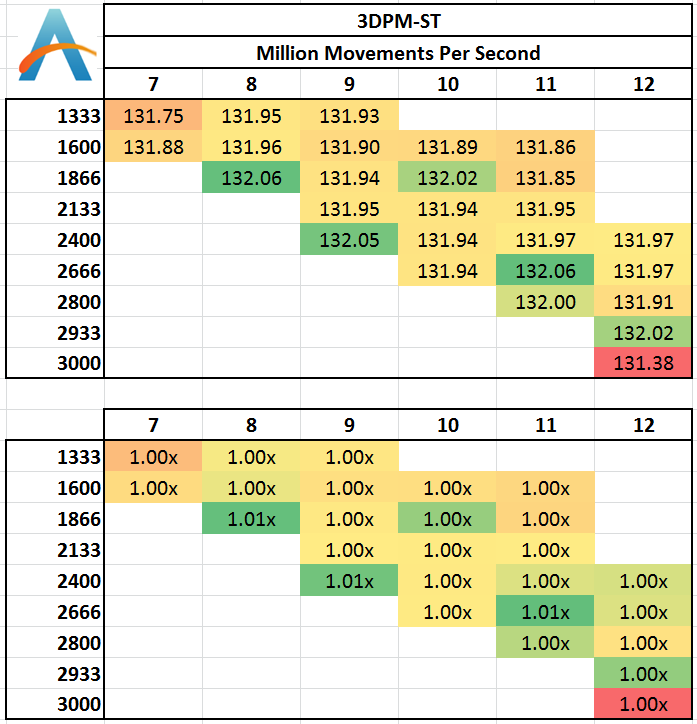
For software that deals with a particle movement at once then discards it, there are very few memory accesses that go beyond the caches into the main DRAM. As a result, we see little differentiation between the memory kits, except perhaps a loose automatic setting with 3000 C12 causing a small decline.
Multi-Threaded:
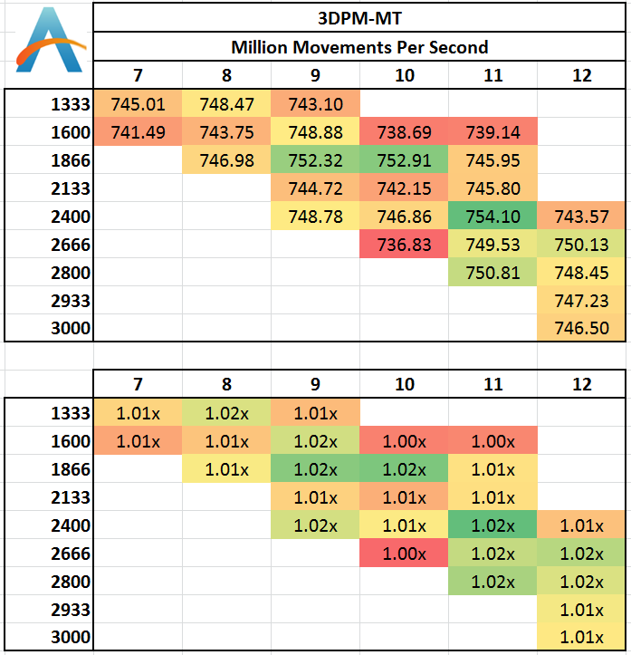
With all the cores loaded, the caches should be more stressed with data to hold, although in the 3DPM-MT test we see less than a 2% difference in the results and no correlation that would suggest a direction of consistent increase.
N-Body Simulation
When a series of heavy mass elements are in space, they interact with each other through the force of gravity. Thus when a star cluster forms, the interaction of every large mass with every other large mass defines the speed at which these elements approach each other. When dealing with millions and billions of stars on such a large scale, the movement of each of these stars can be simulated through the physical theorems that describe the interactions. The benchmark detects whether the processor is SSE2 or SSE4 capable, and implements the relative code. We run a simulation of 10240 particles of equal mass - the output for this code is in terms of GFLOPs, and the result recorded was the peak GFLOPs value.
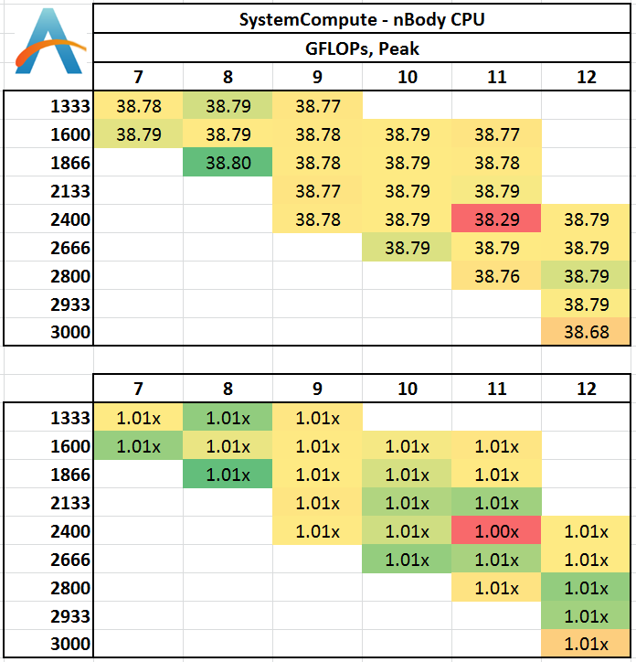
Despite co-interaction of many particles, the fact that a simulation of this scale can hold them all in caches between time steps means that memory has no effect on the simulation.
Grid Solvers - Explicit Finite Difference
For any grid of regular nodes, the simplest way to calculate the next time step is to use the values of those around it. This makes for easy mathematics and parallel simulation, as each node calculated is only dependent on the previous time step, not the nodes around it on the current calculated time step. By choosing a regular grid, we reduce the levels of memory access required for irregular grids. We test both 2D and 3D explicit finite difference simulations with 2n nodes in each dimension, using OpenMP as the threading operator in single precision. The grid is isotropic and the boundary conditions are sinks. We iterate through a series of grid sizes, and results are shown in terms of ‘million nodes per second’ where the peak value is given in the results – higher is better.
Two-Dimensional Grid:
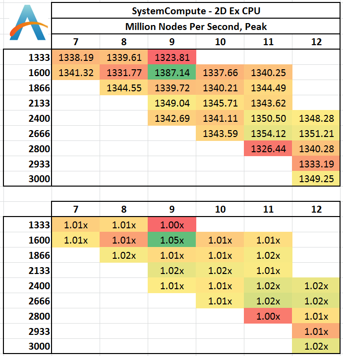
In 2D we get a small bump over at 1600 C9 in terms of calculation speed, with all other results being fairly equal. This would statistically be an outlier, although the result seemed repeatable.
Three Dimensions:
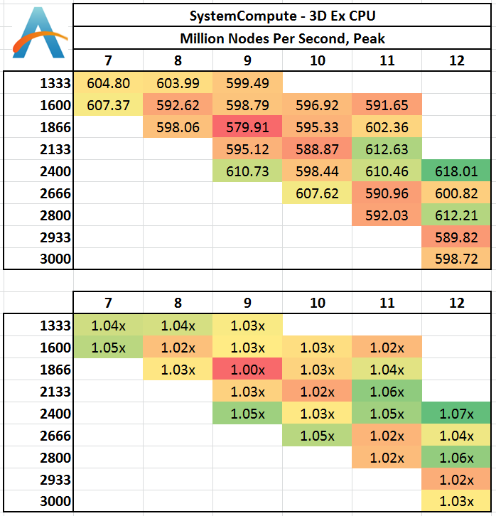
In three dimensions, the memory jumps required to access new rows of the simulation are far greater, resulting in L3 cache misses and accesses into main memory when the simulation is large enough. At this boundary it seems that low CAS latencies work well, as do memory speeds > 2400 MHz. 2400 C12 seems a surprising result.
Grid Solvers - Implicit Finite Difference + Alternating Direction Implicit Method
The implicit method takes a different approach to the explicit method – instead of considering one unknown in the new time step to be calculated from known elements in the previous time step, we consider that an old point can influence several new points by way of simultaneous equations. This adds to the complexity of the simulation – the grid of nodes is solved as a series of rows and columns rather than points, reducing the parallel nature of the simulation by a dimension and drastically increasing the memory requirements of each thread. The upside, as noted above, is the less stringent stability rules related to time steps and grid spacing. For this we simulate a 2D grid of 2n nodes in each dimension, using OpenMP in single precision. Again our grid is isotropic with the boundaries acting as sinks. We iterate through a series of grid sizes, and results are shown in terms of ‘million nodes per second’ where the peak value is given in the results – higher is better.
2D Implicit:
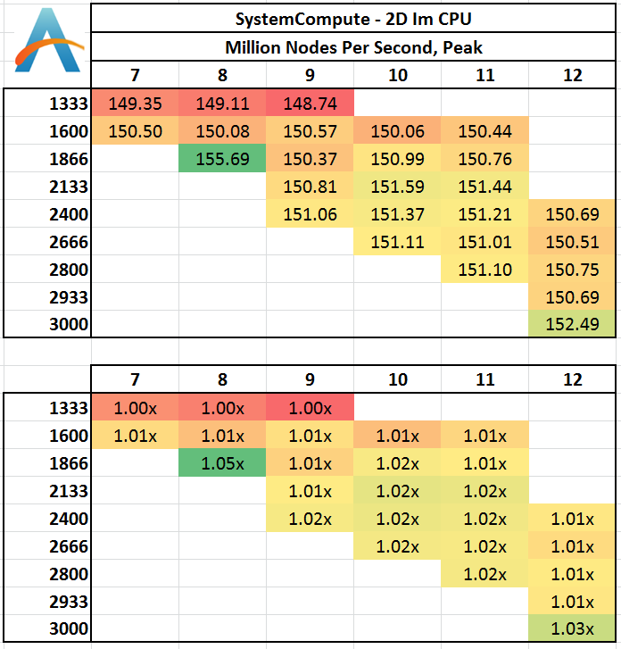
Despite the nature if implicit calculations, it would seem that as long as 1333 MHz is avoided, results are fairly similar. 1866 C8 being a surprise outlier.


89 Comments
View All Comments
gsuburban - Thursday, November 28, 2013 - link
Interesting article however, "Number of Sticks" as noted above would mean what? Is there a performance gain or loss using the same amount of Gigs of the same RAM in say 16GB in two dims versus 16GB of the same using 4 dimms?neal.a.nelson - Sunday, December 8, 2013 - link
That is a reasonable inference, and given the age of the article and date of the last post, probably all you're going to get. For upgrade ability, it's smart to use the two dual-channel slots instead of filling all four with the same amount.htwingnut - Monday, January 20, 2014 - link
Thanks for this testing and article. This shows 1366x768 for resolution. While I understand that this will test the RAM fully, it's also not realistic. I'd like to see results running single 1080p or 3x1080p because that's more real world.melk - Thursday, January 23, 2014 - link
Am I reading this correctly? That there is literally a 1fps difference at best, in both lowest and avg fps?melk - Thursday, January 23, 2014 - link
So we are talking about a ~1 fps difference in real world testing? Wow...dasa43 - Friday, February 28, 2014 - link
To see gains from faster ram the game needs to be cpu limited while most console ports are totally gpu limitedIncreasing resolution just stresses the gpu more further lightning the load on the cpu
Thief & Arma are two cpu limited games that can see big gains from faster ram
Thief benchmarks
http://forums.atomicmpc.com.au/index.php?showtopic...
Arma benchmarks
http://forums.bistudio.com/showthread.php?166512-A...
NordRack2 - Sunday, June 1, 2014 - link
Quote: "Using the older version of WinRAR shows a 31% advantage moving from 1333 C9 to 3000 C12"That's wrongly calculated.
Correct is: ((213.63-163.11)/213.63) × 100% = 24%
cadman777 - Sunday, April 19, 2015 - link
Dear Sir,Do you have an article that explains the basics for RAM, CPU & m/b matching?
I want to learn the basics on this, but all I keep finding are articles like this with bits and pieces, and general explanations of the various components, but no pragmatic explanations on how they work together and how to match them and do the over-clocking between the various components to arrive at a stable system.
Thanx ... Chris
Nickolai - Sunday, August 13, 2017 - link
Is there a similar article for DDR4?