Gigabyte GA-7PESH1 Review: A Dual Processor Motherboard through a Scientist’s Eyes
by Ian Cutress on January 5, 2013 10:00 AM EST- Posted in
- Motherboards
- Gigabyte
- C602
Explicit Finite Difference
For a grid of points or nodes over a simulation space, each point in the space can describe a number of factors relating to the simulation – concentration, electric field, temperature, and so on. In terms of concentration, the material balance gradients are approximated to the differences in the concentrations of surrounding points. Consider the concentration gradient of species C at point x in one dimension, where [C]x describes the concentration of C at x:
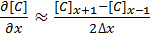 [1]
[1]
The second derivative around point x is determined by combining the half-differences from the adjacent half-points next to x:
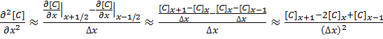 [2]
[2]
Equations [1] and [2] can be applied to the partial differential equation [3] below to reveal a set of linear equations which can be solved.
Fick’s first law for the rate of diffusional mass transport can be applied in three dimensions:
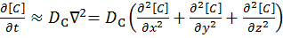 [3]
[3]
where D is the diffusion coefficient of the chemical species, and t is the time. For the dimensional analyses used in this work, the Laplacian is split over the Cartesian dimensions x, y and z.
Dimension transformations are often employed to these simulations to relieve the simulation against scaling factors. The expansion of equation [3] given specific dimension transforms not mentioned here give equation [4] to be solved.
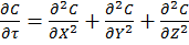 [4]
[4]
The expansion of equation [4] using coefficient collation and expansion by finite differences mentioned in equations [1] and [2] lead to equation [5]:

 [5]
[5]
Equation [5] represents a series of concentrations that can be calculated independently from each other – each concentration can now be solved for each timestep (t) by an explicit algorithm for t+1 from t.
The explicit algorithm is uncommonly used in electrochemical simulation, often due to stability constraints and time taken to simulate. However, it offers complete parallelisation and low thread density – ideal for multi-processor systems and graphics cards – such that these issues should be overcome.
The explicit algorithm is stable when, for equation [4], the Courant–Friedrichs–Lewy condition [6] holds.
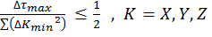 [6]
[6]
Thus the upper bound on the time step is fixed given the minimum grid spacing used.
There are variations of the explicit algorithm to improve this stability, such as the Dufort-Frankel method of considering the concentration at each point as the linear function of time, such that:
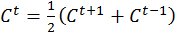 [7]
[7]
However, this method requires knowledge of the concentrations of two steps before the current step, therefore doubling memory usage.
Application to this Review
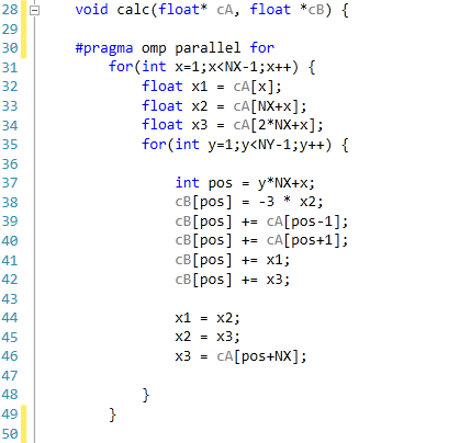
For the purposes of this review, we generate an x-by-x / x-by-x-by-x grid of points with a relative concentration of 1, where the boundaries are fixed at a relative concentration of 0. The grid is a regular grid, simplifying calculations. As each node in the grid is independently calculable from each other, it would be ideal to spawn as many threads as there are nodes. However, each node has to load the data of the nodes of the previous time step around it, thus we restrict parallelization in one dimension and use an iterative loop to restrict memory loading and increase simulation throughput.
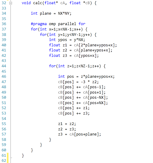
The code was written in Visual Studio C++ 2012 with OpenMP as the multithreaded source. The main functions to do the calculations are as follows.
For 2D:
For 3D:
For our scores, we increase the size of the grid from a 2x2 or 2x2x2 until we hit 2GB memory usage. At each stage, the time taken to repeatedly process the grid over many time steps is calculated in terms of ‘million nodes per second’, and the peak value is used for our results.
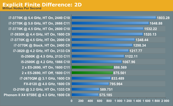
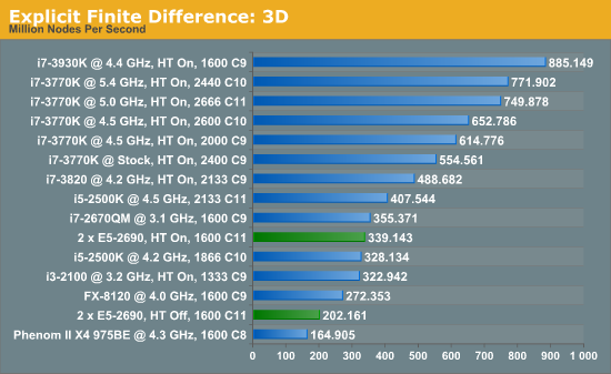
Firstly, the results for our 2D and 3D Explicit Finite Difference simulations are shocking. In 3D, the dual processor system gets beaten by a mobile i7-2670QM (!). In both 2D and 3D, it seems being able to quickly access main memory and L3 caches is top priority. Each processor in the DP machine has to go out to memory when they need a value not in cache, whereas in a single processor machine it can access the L3 cache if the simulation fits wholly in there and the processor can predict which numbers are required next.
Also it should be noted that enabling HyperThreading in 3D gave a better than 50% increase in throughput on the dual processor machine.


64 Comments
View All Comments
dj christian - Monday, January 14, 2013 - link
No please!This article should be a one time only or once every 2 years at most.
nadana23 - Sunday, January 6, 2013 - link
From the looks of results some of the benchmarks are HIGHLY sensitive to effective bandwidth per thread (ie, GDDR5 feeding a GPU stream processor >> DDR3 feeding a Xeon HT core).However - it must be noted that 8x DIMMS is insufficient to achieve full memory bandwidth on Xeon E5 2S!
I'd suggest throwing a pure memory bandwidth test into the mix to make sure you're actually getting the rated number (51.2GB/s)...
http://ark.intel.com/products/64596/Intel-Xeon-Pro...
... as I strongly suspect your memory config is crippling results.
Dell's 12G config guidelines are as good a place as any to start on this :-
http://en.community.dell.com/cfs-file.ashx/__key/c...
Simply removing one E5-2590 and moving to 1-Package, 8 DIMM config may (counter-intuitively) bench(market) faster... for you.
dapple - Sunday, January 6, 2013 - link
Great article, thanks! This is the sort of benchmark I've been wanting to see for quite some time now - simple, brute-force numerics where the code is visible and straightforward. Too many benchmarks are black boxes with processor- and compiler-specific tunes to make manufacturer "X" appear superior to "Y". That said, it would be most illustrative to perform a similar 'mark using vanilla gcc on both MS and *nix OS.daosis - Sunday, January 6, 2013 - link
It is long known issue, when windows does not start after changing hardware, especially GPU (not always so). There is as long known trick so. Just before last "power off" one should replace GPU's own driver with basic microsoft's one. In case of GPU it is "standart Vga adapter" (device manager - update driver - browse my computer - let me pick up). In fact one can replace all specific drivers on OS with similiar basic from MS and then to put this hard drive virtually to any system without any need for fresh install. Mind you, that after first boot it takes some time for OS to find and install specific drivers.jamesf991 - Sunday, January 6, 2013 - link
In the early '70s I was doing very similar simulations using a PDP 11/40 minicomputer. (I can send citations to my publications if anyone is interested.) At Texas Tech and later at Caltech, I simulated systems involving heterogeneous electron transfer kinetics, various chemical reactions in solution, coulostatics, galvanostatics, voltammetry, chronocoulometry, AC voltammetry, migration, double layer effects, solution hydrodynamics (laminar only), etc. Much of this was done on a PDP 11/40, originally with 8K words (= 16K bytes) of core memory. Later the machine was upgraded to 24 K words (!), we got a floating point board, and a hard disk drive (5 M words, IIRC). My research director probably paid in excess of $50K for the hardware. One cute project was to put a simulation "inside" a nonlinear regression routine to solve for electrode kinetic parameters such as k and alpha. Each iteration of the nonlinear solver required a new simulation -- hand-coding the innermost loops using floating point assembly instructions was a big speedup!I wonder how the old PDP would stack up against the 3770?
flynace - Monday, January 7, 2013 - link
Do you guys think that once Haswell moves the VRM on package that someone might do a 2 socket mATX board?Even if it means giving up 2 of the 4 PCIe slots and/or 2 DIMMs per socket it would be nice to have a high core count standard SFF board for those that need just that.
samsp99 - Monday, January 7, 2013 - link
I found this review interesting, but I don't think this board is really targeted at the HPC market. It seems like it would be good as part of a 2U / 12 + 2 drive system, similar to the Dell C2100. It would make a good virtual host, SQL, active web server etc. Having the 3 mSAS connectors would enable 4 drive each without the need for a SAS expander.Servers are designed for 99.999% uptime, remote management, and hands-off operation. To achieve that you need redundent power, UPS, Networking, storage etc. They also require high airflow, which is noisy and not something you want sitting under your desk. Based on that, it makes sense that the MB is intended for sale to system builders not your general build your own enthusiast.
HW manufactuerers are faced with a similar problem to airlines - consumers gravitate to the cheapest price, and so the only real money to be made is selling higher profit margin products to businesses. Servers are where intel etc makes their profits.
For the computational problems the author is trying to solve, to me it would seem to be better to consider:
a) At one point, I think google was using commodity hardware, with custom shelving etc. Assuming the algorithms can be paralleled on different hosts, you shouldn't need the reliability of traditional servers, so why not use a number of commodity systems together, choosing the components that have the best perf/$.
b) There are machines designed for HPC scenarios, such as HPC Systems E5816 that supports 8x Xeon E7-8000 (10 core) processors, or the E4002G8 - that will take 8 nVidia Tesla cards.
c) What about developing and testing the software on cheap worstations, and then when you are sure its ready, buying compute time from Amazon cloud services etc.
babysam - Monday, January 7, 2013 - link
It is quite delighting to look at your review on Anandtech (especially when I am using software and computer configurations of similar nature for my studies), as it is quite difficult for me to evaluate the performance gain of "real-life" software (i.e. science oriented in my case) on new hardware before buying.From what I have seen in your code segments provided (especially for the n-body simulation part) , there are large amount of floating-point divisions. Is there any possibility that the code is not only limited by the cache size(and thrashing), but by the limited throughput of the floating-point divider? (i.e. The performance degradations when HT is enabled may also be caused by the competition of the two running threads on the only floating-point divider in the core)
SanX - Tuesday, January 8, 2013 - link
if you post zipped sources and exes for anyone to follow, learn, play, argue and eventually improve.I'd also preferred to see Fortran sources and benchmarks when possible.
Intel/AMD should start promote 2/4/8 socket monster mobos for enthusiasts and then general public since this is the beginning of the infinite in time era for multiprocessing.
Also where are games benchmarks like for example GTA4 which benefits a lot from multicores as well as from GPUs?
IanCutress - Wednesday, January 9, 2013 - link
The n-body simulations are part of the C++ AMP example page, free for everyone to use. The rest of the code is part of a benchmark package I'm creating, hence I only give the loops in the code. Unfortunately I know no Fortran for benchmarks.Most mainstream users (i.e. gamers) still debate whether 4 or 6 cores are even necessary, so moving to 2P/4P/8P is a big leap in that regard. Enthusiasts can still get the large machines (a few folders use quad AMD setups) if they're willing to buy from ebay which may not always be wholly legal. You may see 2P/4P/8P becoming more mainstream when we start to hit process node limits.
Ian