Gigabyte GA-7PESH1 Review: A Dual Processor Motherboard through a Scientist’s Eyes
by Ian Cutress on January 5, 2013 10:00 AM EST- Posted in
- Motherboards
- Gigabyte
- C602
Two Dimensional Implicit Finite Difference
The ‘Finite Difference’ part of this computational grid solver means that the derivation of this method is similar to that shown in the Explicit Finite Difference method on the previous page. We are presented with the following equation which explains Fick’s first law of diffusion for mass transport in three dimensions:
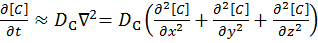 [8]
[8]
The implicit method takes the view that the concentrations at time t+1 are a series of unknowns, and the equations are thus coupled into a series of simultaneous equations with an equal set of unknowns, which must be solved together:
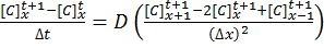 [9]
[9]
 [10]
[10]
The implicit method is algorithmically more complex than the explicit method, but does offer the advantage of unconditional stability with respect to time.
The Alternating Direction Implicit (ADI) Method
For a system in two dimensions (labelled r and z), such as a microdisk simulation, the linear system has to be solved in both directions using Fick’s Laws:
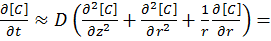
 [11]
[11]
The alternating direction implicit (ADI) method is a straightforward solution to solving what are essentially two dimensional simultaneous equations whilst retaining a high degree of algorithm stability.
ADI splits equation [11] into two half time steps – by treating one dimension explicitly and the other dimension implicitly in the same half time step. Thus the explicit values known in one direction are fed into the series of simultaneous equations to solve the other direction. For example, using the r direction explicitly to solve the z direction implicitly:
 [12]
[12]
 [13]
[13]
By solving equation [13] for the concentrations in the z direction, the next half time step concentrations can be calculated for the r direction, and so on until the desired time in simulation is achieved. These time step equations are solved using the Thomas Algorithm for tri-diagonal matrices.
Application to this Review
For the purposes of this review, we generate an x-by-x grid of points with a relative concentration of 1, where the boundaries are fixed at a relative concentration of 0. The grid is a regular grid, simplifying calculations. The nature of the simulation allows that for each half-time step to focus on calculating in one dimension, for a simulation of x-by-x nodes we can spawn x threads as adjacent rows/columns (depending on direction) are independent. These threads, in comparison to the explicit finite difference, are substantially bulkier in terms of memory usage.
The code was written in Visual Studio C++ 2012 with OpenMP as the multithreaded source. The main function to do the calculations is as follows.
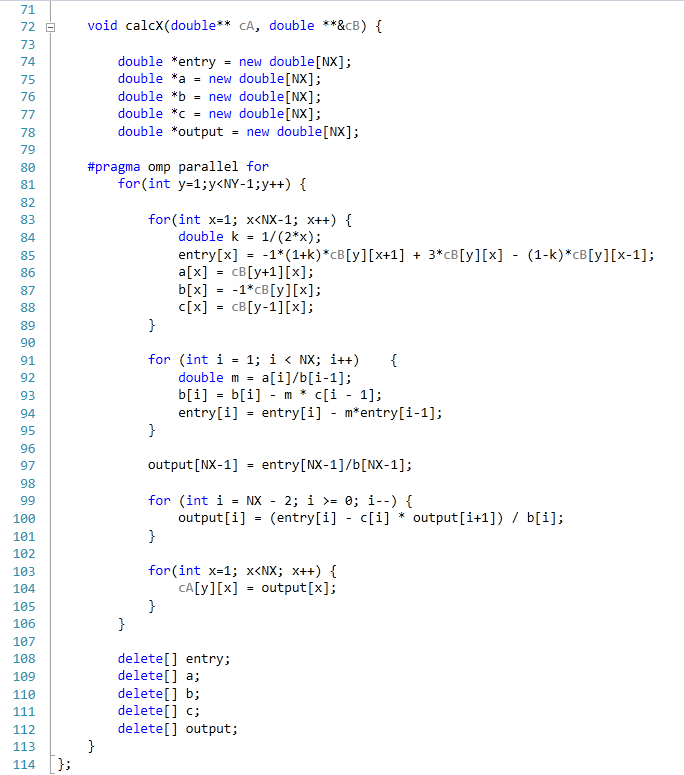
For our scores, we increase the size of the grid from a 2x2 until we hit 2GB memory usage. At each stage, the time taken to repeatedly process the grid over many time steps is calculated in terms of ‘million nodes per second’, and the peak value is used for our results.
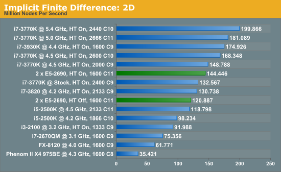
Previously where the explicit 2D method was indifferent to HyperThreading and the explicit 3D method was very sensitive; the implicit 2D is a mix of both. There are still benefits to be had from enabling HyperThreading. Nevertheless, the line between single processor systems and dual processors is being blurred a little due to the different speeds of the SP results, but in terms of price/performance, the DP system is at the wrong end.


64 Comments
View All Comments
Hulk - Saturday, January 5, 2013 - link
I had no idea you were so adept with mathematics. "Consider a point in space..." Reading this brought me back to Finite Element Analysis in college! I am very impressed. Being a ME I would have preferred some flow models using the Navier-Stokes equations, but hey I like chemistry as well.IanCutress - Saturday, January 5, 2013 - link
I never did any FEM so wouldn't know where to start. The next angle of testing would have been using a C++ AMP Fluid Dynamics Simulation and adjusting the code from the SDK example like with the n-Body testing. If there is enough interest, I could spend a few days organising it for the normal motherboard reviews :)Ian
mayankleoboy1 - Saturday, January 5, 2013 - link
How the frick did you get the i7-3770K to *5.4GHZ* ? :shock:How the frick did you get the i7-3770K to *5.0GHZ* ? :shock:
IanCutress - Saturday, January 5, 2013 - link
A few members of the Overclock.net HWBot team helped testing by running my benchmark while they were using DICE/LN2/Phase Change for overclocking contests (i.e. not 24/7 runs). The i7-3770K will go over 7 GHz if (a) you get a good chip, (b) cool it down enough, and (c) know what you are doing. If you're interested in competitive overclocking, head over to HWBot, Xtreme Systems or Overclock.net - there are plenty of people with info to help you get started.Ian
JlHADJOE - Tuesday, January 8, 2013 - link
The incredible performance of those overclocked Ivy bridge systems here really hammers home the importance of raw IPC. You can spend a lot of time optimizing code, but IPC is free speed when it's available.jd_tiger - Saturday, January 5, 2013 - link
http://www.youtube.com/watch?v=Ccoj5lhLmSQsmonsees - Saturday, January 5, 2013 - link
You might try modifying your algorithm to pin the data to a specific core (therefore cache) to keep the thrashing as low as possible. Google "processor affinity c++". I will admit this adds complexity to your straightforward algorithm. In C#, I would use a parallel loop with a range partition to do it as a starting point: http://msdn.microsoft.com/en-us/library/dd560853.a...nickgully - Saturday, January 5, 2013 - link
Mr. Cutress,Do you think with all the virtualized CPU available, researchers will still build their own system as it is something concrete to put into a grant application, versus the power-by-the-hour of cloud computing?
Thanks.
IanCutress - Saturday, January 5, 2013 - link
We examined both scenarios. Our university had cluster time to buy, and there is always the Amazon cloud. In our calculation, getting a 16 thread machine from Dell paid for itself in under six months of continuous running, and would not require a large adjustment in the way people were currently coding (i.e. staying in Windows rather than moving to Linux), and could also be passed down the research group when newer hardware is released.If you are using production level code and manipulating it each time to get results, and you can guarantee the results will be good each time, then power-by-the-hour could work. As we were constantly writing and testing new code for different scenarios, the build/buy your own workstation won out. Having your own system also helps in building GPU codes, if you want to buy a better GPU card it is easier to swap out rather than relying on a cloud computing upgrade.
Ian
jtv - Sunday, January 6, 2013 - link
One big consideration is who the researchers are. I work in x-ray spectroscopy (as a computational theorist). Experimentalists in this field use some of our codes without wanting to bother with having big computational resources. We have looked at trying to provide some of our codes through some cloud-based service so that it can be used on demand.Otherwise I would agree with Ian's reply. When I'm improving code, debugging code, or trying to implement new theoretical approaches I absolutely want my own hardware to do it on.