Gigabyte GA-7PESH1 Review: A Dual Processor Motherboard through a Scientist’s Eyes
by Ian Cutress on January 5, 2013 10:00 AM EST- Posted in
- Motherboards
- Gigabyte
- C602
Brownian Motion
When chemicals move around in the air, or dissolved in a liquid, or even travelling through a solid, they diffuse from an area of high concentration to low concentration, or follow Le Chatelier’s principle if an external force is applied. Typically this movement is described via an overall statistical shift, expressed as a partial differential equation. However, if we were to pick out an individual chemical and observe its movements, we would see that it moves randomly according to thermal energy – at every step it moves in a random direction until an external force (such as another chemical gets in the way) is encountered. If we sum up the movements of millions or billions of such events, we get the gradual motion explained by statistics.
The purpose of Brownian motion simulation is to calculate what happens to individual chemicals in circumstances where the finite motion is what dictates the activity occurring. For example, experiments dealing with single molecule detection rely on how a single molecule moves, or during deposition chemistry, the movement of individual chemicals will dictate how a surface achieves deposition in light of other factors. The movement of the single particle is often referred to a Random Walk (of which there are several types).
There are two main differences between a random-walk simulation and the finite difference methods used over the previous pages. The first difference is that in a random walk simulation each particle in the simulation is modelled as a point particle, completely independent in its movement with respect to other particles in the simulation (the diffusion coefficient in this context is indirectly indicative of the medium through which the particle is travelling through). With point particles, the interactions at boundaries can be quantized with respect to the time in simulation. From the perspective of independent particles, we can utilise various simulation techniques designed for parallel problems, such as multi-CPU analysis or using GPUs. To an extent, this negates various commentaries which criticise the random-walk method for being exceedingly slow.
The second difference is the applicability to three dimensional simulations. Previous methods for tackling three dimensional diffusion (in the field I was in) have relied on explicit finite difference calculation of uncomplicated geometries, which result in large simulation times due to the unstable nature of the discretisation method. The alternating direction implicit finite difference method in three dimensions has also been used, but can suffer from oscillation and stability issues depending on the algorithm method used. Boundary element simulation can be mathematically complex for this work, and finite element simulation can suffer from poor accuracy. The random-walk scenario is adaptable to a wide range of geometries and by simple redefinition of boundaries and/or boundary conditions, with little change to the simulation code.
In a random walk simulation, each particle present in the simulation moves in a random direction at a given speed for a time step (determined by the diffusion coefficient). Two factors computationally come into play – the generation of random numbers, and the algorithm for determining the direction in which the particle moves.
Random number generation is literally a minefield when first jumped into. Anyone with coding experience should have come across a rand() function that is used to quickly (and messily) generate a random number. This number as a function of the language library repeats itself fairly regularly, often within 2^15 (32768) steps. If a simulation is dealing with particles doing 100,000 steps, or billions of particles, this random number generator is not sufficient. For both CPU and GPU there are a number of free random number generators available, and ones like the Mersenne Twister are very popular. We use the Ranq1 random number generator found in Numerical Recipes 3rd Edition: The Art of Scientific Computing by Press et al., which features a quick generation which has a repeated stepping of ~1.8 x 10^19. Depending on the type of simulation contraints, in order to optimize the speed of the simulation, the random numbers can be generated in an array before the threads are issued and the timers started then sent through the function call. This uses additional memory, but is observed to be quicker than generating random numbers on the fly in the movement function itself.
Random Movement Algorithms
Trying to generate random movement is a little trickier than random numbers. To move a certain distance from an original point, the particle could end up anywhere on the surface of a sphere. The algorithm to generate such movement is not as trivial as a random axial angle followed by a random azimuth angle, as this generates movement biased at the poles of a sphere. By doing some research, I published six methods I had found for generating random points on the surface of a sphere.
For completeness, the notation x ~ U(0,1] means that x is a uniformly generated single-ended random number between 0 and 1.
(i) Cosine Method
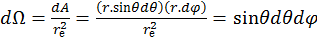
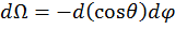
In spherical polar coordinates, the solid angle of a sphere, Ω, is defined as the area A covered by that angle divided by the square of the radius, re, as shown in equation 14. The rate of change of this angle with respect to the area at constant radius gives the following set of equations:
 [14]
[14]
 [15]
[15]
 [16]
[16]
Thus Θ has a cosine weighting. This algorithm can then be used by following these steps:
Generate 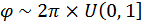 [17]
[17]
Generate 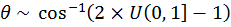 [18]
[18]
 [19]
[19]
 [20]
[20]
 [21]
[21]
Computationally, 2π can be predefined as a constant, and thus does not require a multiplication every time it is used.
(ii) Normal-Deviate Method
As explained by Knuth, each x, y and z coordinate is randomly generated from a normal distribution with a mean of 0 and variance of 1. The result is normalised to the surface of the sphere to obtain a uniform distribution on the surface. The following equations describe this method, where λis the normalisation factor:
Let u, v, w ~ N(0,1), λ = Rm / sqrt(u2+v2+w2) [22]
x = uλ, y = vλ, z = wλ [23]
It should be noted that the generation of normally distributed random numbers requires an element of rejection, and thus generating normal random numbers takes significantly longer than generating uniform random numbers.
(iii) Hypercube rejection method
Similar to the normal-deviate method, but each ordinate is uniformly randomly distributed on [-1, 1] (calculated as 2 x U(0,1]-1). Compute the square root of the sum of squares, and if this value is greater than 1, the triplet is rejected. If this value is below 1, the vector is normalised and scaled to Rm.
Generate u, v, w ~ 2 * U(0,1] - 1 [24]
Let s2 = u2 + v2 + w2; if s>1, reject, else λ = Rm/s [25]
x = uλ, y = vλ, z = wλ [26]
As this method requires comparison and rejection, the chance of a triplet being inside the sphere as required is governed by the areas of a cube and sphere, such that 6/3.141 ≈ 1.910 triplets are required to achieve one which passes comparison.
(iv) Trigonometric method
This method is based on the fact that particles will be uniformly distributed on the sphere in one axis. The proof of this has been published in peer reviewed journals. The uniform direction, in this case Z, is randomly generated on [-Rm, Rm] to find the circle cross section at that point. The particle is then distributed at a random angle on the XY plane due to the constraint in Z.
Generate z ~ 2 x Rm x U(0,1] - Rm [27]
Generate α ~ 2π x U(0,1] [28]
Let r = sqrt(Rm2 – z2) [29]
x = r cos(α) [30]
y = r sin(α) [31]
(v) Two-Dimensional rejection method
By combining methods (iii) and (iv), a form of the trigonometric method can be devised without the use of trigonometric functions. Two random numbers are uniformly distributed along [-1, 1]. If the sum of squares of the two numbers is greater than 1, reject the doublet. If accepted, the ordinates are calculated based on the proof that points in a single axis are uniformly distributed:
Generate u, v ~ 2 x U(0,1] - 1 [32]
Let s = u2 + v2; if s > 1, reject. [33]
Let a = 2 x sqrt(1-s); k = a x Rm [34]
x = ku, y = kv, z = (2s-1)Rm [35]
Use of this method over the trigonometric method described in (iii) is dependent on whether the trigonometric functions of the system are slower than the combined speed of rejection and regeneration of the random numbers.
(vi) Bipyramidal Method
For completeness, the bipyramidal diffusion modelis also included. This method generates a random whole number between 0 and 5 inclusive, which dictates a movement in an axis, either positive or negative relative to the starting position. As a result, the one-dimensional representation of the random-walk, as shown in Figure 3, is played out in each of the three dimensions, and any particles that would have ended up outside the bipyramid from methods (i-v) would now be inside the pyramid.
The method for bipyramidal diffusion is shown below:
Generate  where
where  is the floor function
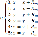 [36]
[36]
This method is technically the computationally least expensive in terms of mathematical functions, but due to equation [36], requires a lot of ‘if’ type comparison statements and the speed of these will determine how fast the algorithm is.
Results
The Brownian motion tests are something I have been doing with motherboard reviews for over twelve months in the form of my 3DPM (Three-Dimensional Particle Movement) test in both single threaded and multithreaded form. The simulation generates a number of particles, iterates them through a number of steps, and then checks the time to see if 10 seconds have passed. If the 10 seconds are not up, it goes through another loop. Results are then expressed in the form of million particle movements per second.
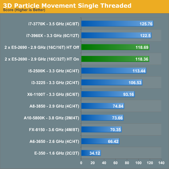
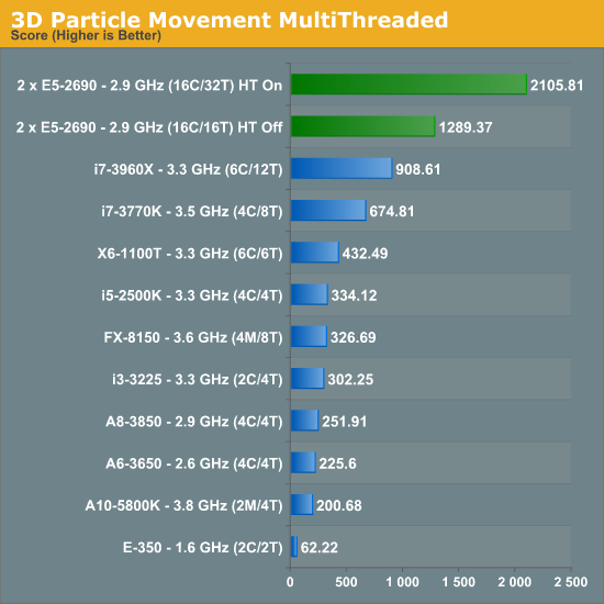
Due to the nature of the simulation, absolutely no memory access are needed during computation - there is a small element at the end for addition. This makes the DP system excellent for this type of work. Perhaps unsurprisingly we see no change in our single threaded version with HyperThreading on or off. However with the multithreaded version, HyperThreading gets a massive 63.3% boost.
Abusing GPUs
Back when I was researching these methods and implementing them on GPUs, for method (iv), the fastest method, the following results were achieved:
Athlon X2 5050e, 2.6 GHz (2C/2T): 32.38
Dual Xeon E5520, 2.23 GHz (8C/16T): 230.63
NVIDIA Quadro 580, 32 CUDA Cores: 1041.80
NVIDIA GTX 460, 336 CUDA Cores: 13602.94
When the simulation is embarrassingly parallel like this one, GPUs make a lot of difference. I recently rewrote method (iv) in C++ AMP and ran it on a i7-3770K at stock with a HD7970 also at stock, paired with 2400 C9 memory. It gave a result of 73654.32.


64 Comments
View All Comments
Hakon - Saturday, January 5, 2013 - link
Thank you for the detailed answer. I very much appreciate your article and hope to see more stuff like this on Anandtech.What I meant regarding to NUMA is the following. When you have a dual socket Xeon you have two memory controllers. The first time you 'touch' a memory location it is assigned to the memory controller of the CPU that runs the current thread. This assignment is in general permanent and all further memory read/writes to that location will be served by that memory controller.
If you first-touch (e.g. initialize the array to zero) using one thread, then the whole array is assigned to one of the two memory controllers. When you then run the multi-threaded code on that array one memory controller is idle while the other is oversubscribed since it has to serve both CPUs.
In contrast, if you first-touch your array in an OpenMP loop and use the same access pattern as in the algorithm, you will benefit from both memory controllers later on. In this case your large array is correctly 'distributed' over both memory controllers.
This kind of memory layout optimization becomes extremely important when you deal with quad socket Opterons. You then have eight memory controllers. A NUMA aware code is therefore up to eight times as fast since it utilizes all memory controllers.
toyotabedzrock - Saturday, January 5, 2013 - link
You should go ask the people on the assembly boards for help with making your code faster.They are very friendly compared to a Linux kernel devs, I think they just enjoy the acknowledgement that they still exist and are useful.
snajpa - Saturday, January 5, 2013 - link
Blame the scheduler. Neither Windows nor linux can effectively handle larger NUMA systems. It randomly moves the process across the physical hardware.psyq321 - Sunday, January 6, 2013 - link
Hmm, this is definitely not true at least for Windows Server 2008 R2 / Windows 7, and I am sure it holds true for some versions of Linux (I am not a Linux expert).Windows Server 2008 R2 / Windows 7 scheduler will try to match the memory allocations (even if they are not tagged for a specific NUMA node) with the NUMA node the process/thread resides on, and they will not move a thread to a foreign NUMA node unless if that has been explicitly requested by the application (by setting the thread affinity)
Of course, without explicit NUMA node tagging when doing allocations, application code is the main culprit for not respecting the NUMA layout (e.g. creating bunch of threads, allocating memory from one of them - and then pinning the threads to different CPUs - you will have lots of LLC requests from remote DRAM because memory was a-priori allocated on one node).
For this - some sane coding helps a lot, here:
http://www.dimkovic.com/node/15
I describe how I extracted more than double performance by careful memory allocation (NUMA-aware) - please note that neither Windows nor Linux scheduler is able to cope with code which is not written to be NUMA aware and it is using large number of threads that are supposed to run on all CPUs.. Simply put, application writer will have to manage memory allocation and usage in the way so that there are as little remote DRAM requests as possible.
snajpa - Sunday, January 6, 2013 - link
About Windows scheduler - I only worked with Windows XP, now I don't have any reason to work with Win anymore, so what you say probably is really true. As for the linux versions - well, long story short, CFS sucks and everyone knows it - this is particularly noticeable if you have fully virtualized VMs which appear as one single process at the host system - the process is randomly swapped between CPU cores and even CPU dies.... sad story. That's why people have to pin their CPUs to their tasks manually.psyq321 - Sunday, January 6, 2013 - link
Ah, XP - that explains it. True, XP did not care about NUMA at all.Windows Server 2008 / Vista introduced NUMA-aware memory allocations, and changed their CPU scheduler so it does not move the thread across NUMA nodes. They will also try to allocate the memory from the thread's own NUMA node when legacy VirtualAlloc etc. APIs are used.
Windows Server 2008 R2 / Windows 7 introduced the concept of CPU groups - allowing more than 64 CPUs. This does require some adaptation of the application, as old threading APIs only work with 64-bit affinity bitmask which only allowed recognizing 64 CPUs. Now, there is a new set of APIs that work with GROUP_AFFINITY structure, allowing control of CPU groups, too. However, this needs explicit change of the legacy process/threading APIs to the new ones.
Furthermore, none of the above can replace some manual intervention*- while Windows scheduler will, indeed, respect NUMA node boundaries and not try to mess around with moving threads across them - it still does not know what the underlying algorithm wants to do.
* There is no need to set the thread affinity to one specific CPU anymore - this prevents running the thread on any other CPU completely. Instead, there is an API called SetThreadIdealProcessor(Ex) which signals Windows scheduler that thread >should< run on that particular CPU - but, under certain circumstances the scheduler can move the thread somewhere else - if the CPU is completely taken away by some other thread/process. Scheduler will try to move the thread as close as possible - to the next core in the socket, for example - or to the next core in the group (group is always contained within a NUMA node).
You can, however, absolutely forbid Windows scheduler from passing the thread to another NUMA node under any circumstances by simply getting the said NUMA node affinity mask (GetNumaNodeProcessorMask(Ex)) and setting this affinity as a thread affinity. This + setting the "ideal" processor still gives Windows scheduler some headroom to move the thread to another core if it is found to be better in a given moment, but it will not even attempt to cross the NUMA boundary in any case whatsoever.
lmcd - Monday, January 7, 2013 - link
While I haven't personally researched them, there are tons of other schedulers that have been written for Linux and I'm certain *at least* one of them is more fitting to this line of work. I've heard of alternatives like BFS and the Linux kernel is so widely used I'm sure there's a gem out there for this application.toyotabedzrock - Saturday, January 5, 2013 - link
Have you ever tried the Intel Math Kernel Library? It might speed up some of the equations. It also hands off work to the Intel MIC card if it thinks it will speed it up.http://software.intel.com/en-us/intel-mkl/
KAlmquist - Saturday, January 5, 2013 - link
The GA-7PESH1 motherboard is $855, and the CPU's are $2020 each, which adds up to $4895. On tasks which don't parallelize well, you can get similar performance from the i7-3770K, which costs an order of magnitude less. (Prices: i7-3770K $320, ASRock Z77 Extreme6 motherboard $152, total from motherboard and CPU $472.) On tasks which parallelize well enough that they can be run on a GPU, the system with the GA-7PESH1 will beat the i7-3770K, but will be crushed by a midrange GPU. So the price/performance of this system is pretty bad unless you throw just the right workload at it.The motherboard price from super-laptop-parts dot com, and the other prices are from a major online retailer that I won't name in order to get around the spam filter.
Death666Angel - Saturday, January 5, 2013 - link
So, your 3770K has ECC memory or VT-D, TXT etc.?