Gigabyte GA-7PESH1 Review: A Dual Processor Motherboard through a Scientist’s Eyes
by Ian Cutress on January 5, 2013 10:00 AM EST- Posted in
- Motherboards
- Gigabyte
- C602
Brownian Motion
When chemicals move around in the air, or dissolved in a liquid, or even travelling through a solid, they diffuse from an area of high concentration to low concentration, or follow Le Chatelier’s principle if an external force is applied. Typically this movement is described via an overall statistical shift, expressed as a partial differential equation. However, if we were to pick out an individual chemical and observe its movements, we would see that it moves randomly according to thermal energy – at every step it moves in a random direction until an external force (such as another chemical gets in the way) is encountered. If we sum up the movements of millions or billions of such events, we get the gradual motion explained by statistics.
The purpose of Brownian motion simulation is to calculate what happens to individual chemicals in circumstances where the finite motion is what dictates the activity occurring. For example, experiments dealing with single molecule detection rely on how a single molecule moves, or during deposition chemistry, the movement of individual chemicals will dictate how a surface achieves deposition in light of other factors. The movement of the single particle is often referred to a Random Walk (of which there are several types).
There are two main differences between a random-walk simulation and the finite difference methods used over the previous pages. The first difference is that in a random walk simulation each particle in the simulation is modelled as a point particle, completely independent in its movement with respect to other particles in the simulation (the diffusion coefficient in this context is indirectly indicative of the medium through which the particle is travelling through). With point particles, the interactions at boundaries can be quantized with respect to the time in simulation. From the perspective of independent particles, we can utilise various simulation techniques designed for parallel problems, such as multi-CPU analysis or using GPUs. To an extent, this negates various commentaries which criticise the random-walk method for being exceedingly slow.
The second difference is the applicability to three dimensional simulations. Previous methods for tackling three dimensional diffusion (in the field I was in) have relied on explicit finite difference calculation of uncomplicated geometries, which result in large simulation times due to the unstable nature of the discretisation method. The alternating direction implicit finite difference method in three dimensions has also been used, but can suffer from oscillation and stability issues depending on the algorithm method used. Boundary element simulation can be mathematically complex for this work, and finite element simulation can suffer from poor accuracy. The random-walk scenario is adaptable to a wide range of geometries and by simple redefinition of boundaries and/or boundary conditions, with little change to the simulation code.
In a random walk simulation, each particle present in the simulation moves in a random direction at a given speed for a time step (determined by the diffusion coefficient). Two factors computationally come into play – the generation of random numbers, and the algorithm for determining the direction in which the particle moves.
Random number generation is literally a minefield when first jumped into. Anyone with coding experience should have come across a rand() function that is used to quickly (and messily) generate a random number. This number as a function of the language library repeats itself fairly regularly, often within 2^15 (32768) steps. If a simulation is dealing with particles doing 100,000 steps, or billions of particles, this random number generator is not sufficient. For both CPU and GPU there are a number of free random number generators available, and ones like the Mersenne Twister are very popular. We use the Ranq1 random number generator found in Numerical Recipes 3rd Edition: The Art of Scientific Computing by Press et al., which features a quick generation which has a repeated stepping of ~1.8 x 10^19. Depending on the type of simulation contraints, in order to optimize the speed of the simulation, the random numbers can be generated in an array before the threads are issued and the timers started then sent through the function call. This uses additional memory, but is observed to be quicker than generating random numbers on the fly in the movement function itself.
Random Movement Algorithms
Trying to generate random movement is a little trickier than random numbers. To move a certain distance from an original point, the particle could end up anywhere on the surface of a sphere. The algorithm to generate such movement is not as trivial as a random axial angle followed by a random azimuth angle, as this generates movement biased at the poles of a sphere. By doing some research, I published six methods I had found for generating random points on the surface of a sphere.
For completeness, the notation x ~ U(0,1] means that x is a uniformly generated single-ended random number between 0 and 1.
(i) Cosine Method
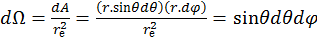
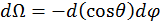
In spherical polar coordinates, the solid angle of a sphere, Ω, is defined as the area A covered by that angle divided by the square of the radius, re, as shown in equation 14. The rate of change of this angle with respect to the area at constant radius gives the following set of equations:
 [14]
[14]
 [15]
[15]
 [16]
[16]
Thus Θ has a cosine weighting. This algorithm can then be used by following these steps:
Generate 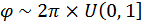 [17]
[17]
Generate 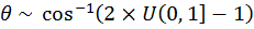 [18]
[18]
 [19]
[19]
 [20]
[20]
 [21]
[21]
Computationally, 2π can be predefined as a constant, and thus does not require a multiplication every time it is used.
(ii) Normal-Deviate Method
As explained by Knuth, each x, y and z coordinate is randomly generated from a normal distribution with a mean of 0 and variance of 1. The result is normalised to the surface of the sphere to obtain a uniform distribution on the surface. The following equations describe this method, where λis the normalisation factor:
Let u, v, w ~ N(0,1), λ = Rm / sqrt(u2+v2+w2) [22]
x = uλ, y = vλ, z = wλ [23]
It should be noted that the generation of normally distributed random numbers requires an element of rejection, and thus generating normal random numbers takes significantly longer than generating uniform random numbers.
(iii) Hypercube rejection method
Similar to the normal-deviate method, but each ordinate is uniformly randomly distributed on [-1, 1] (calculated as 2 x U(0,1]-1). Compute the square root of the sum of squares, and if this value is greater than 1, the triplet is rejected. If this value is below 1, the vector is normalised and scaled to Rm.
Generate u, v, w ~ 2 * U(0,1] - 1 [24]
Let s2 = u2 + v2 + w2; if s>1, reject, else λ = Rm/s [25]
x = uλ, y = vλ, z = wλ [26]
As this method requires comparison and rejection, the chance of a triplet being inside the sphere as required is governed by the areas of a cube and sphere, such that 6/3.141 ≈ 1.910 triplets are required to achieve one which passes comparison.
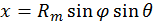
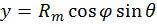
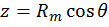
(iv) Trigonometric method
This method is based on the fact that particles will be uniformly distributed on the sphere in one axis. The proof of this has been published in peer reviewed journals. The uniform direction, in this case Z, is randomly generated on [-Rm, Rm] to find the circle cross section at that point. The particle is then distributed at a random angle on the XY plane due to the constraint in Z.
Generate z ~ 2 x Rm x U(0,1] - Rm [27]
Generate α ~ 2π x U(0,1] [28]
Let r = sqrt(Rm2 – z2) [29]
x = r cos(α) [30]
y = r sin(α) [31]
(v) Two-Dimensional rejection method
By combining methods (iii) and (iv), a form of the trigonometric method can be devised without the use of trigonometric functions. Two random numbers are uniformly distributed along [-1, 1]. If the sum of squares of the two numbers is greater than 1, reject the doublet. If accepted, the ordinates are calculated based on the proof that points in a single axis are uniformly distributed:
Generate u, v ~ 2 x U(0,1] - 1 [32]
Let s = u2 + v2; if s > 1, reject. [33]
Let a = 2 x sqrt(1-s); k = a x Rm [34]
x = ku, y = kv, z = (2s-1)Rm [35]
Use of this method over the trigonometric method described in (iii) is dependent on whether the trigonometric functions of the system are slower than the combined speed of rejection and regeneration of the random numbers.
(vi) Bipyramidal Method
For completeness, the bipyramidal diffusion modelis also included. This method generates a random whole number between 0 and 5 inclusive, which dictates a movement in an axis, either positive or negative relative to the starting position. As a result, the one-dimensional representation of the random-walk, as shown in Figure 3, is played out in each of the three dimensions, and any particles that would have ended up outside the bipyramid from methods (i-v) would now be inside the pyramid.
The method for bipyramidal diffusion is shown below:
Generate 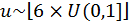 where
where  is the floor function
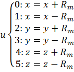 [36]
[36]
This method is technically the computationally least expensive in terms of mathematical functions, but due to equation [36], requires a lot of ‘if’ type comparison statements and the speed of these will determine how fast the algorithm is.
Results
The Brownian motion tests are something I have been doing with motherboard reviews for over twelve months in the form of my 3DPM (Three-Dimensional Particle Movement) test in both single threaded and multithreaded form. The simulation generates a number of particles, iterates them through a number of steps, and then checks the time to see if 10 seconds have passed. If the 10 seconds are not up, it goes through another loop. Results are then expressed in the form of million particle movements per second.
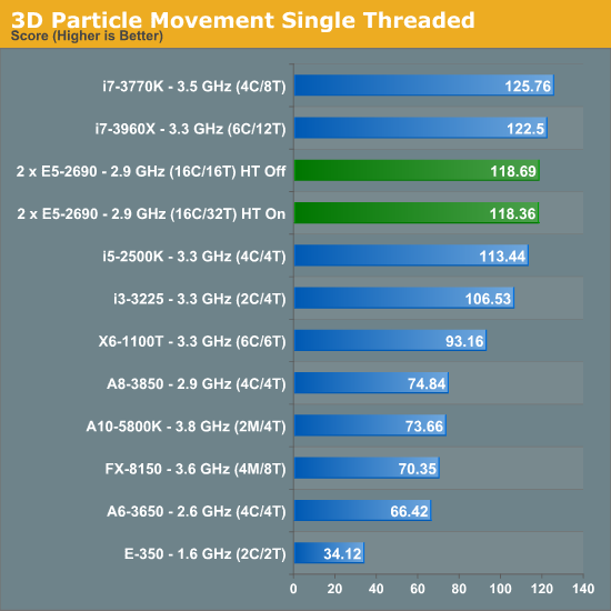
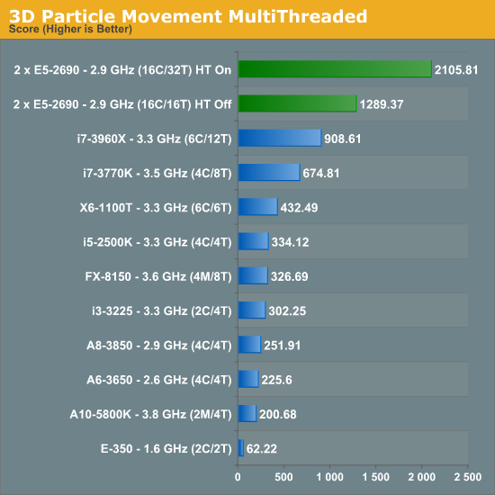
Due to the nature of the simulation, absolutely no memory access are needed during computation - there is a small element at the end for addition. This makes the DP system excellent for this type of work. Perhaps unsurprisingly we see no change in our single threaded version with HyperThreading on or off. However with the multithreaded version, HyperThreading gets a massive 63.3% boost.
Abusing GPUs
Back when I was researching these methods and implementing them on GPUs, for method (iv), the fastest method, the following results were achieved:
Athlon X2 5050e, 2.6 GHz (2C/2T): 32.38
Dual Xeon E5520, 2.23 GHz (8C/16T): 230.63
NVIDIA Quadro 580, 32 CUDA Cores: 1041.80
NVIDIA GTX 460, 336 CUDA Cores: 13602.94
When the simulation is embarrassingly parallel like this one, GPUs make a lot of difference. I recently rewrote method (iv) in C++ AMP and ran it on a i7-3770K at stock with a HD7970 also at stock, paired with 2400 C9 memory. It gave a result of 73654.32.


64 Comments
View All Comments
toyotabedzrock - Saturday, January 5, 2013 - link
There is a large number of very smart people on Google+. You really should come join us.JlHADJOE - Tuesday, January 8, 2013 - link
Of course there are lots of smart people on G+! You're all google employees right? =PActivate: AMD - Saturday, January 5, 2013 - link
As a fellow chemist, I must say that you have to be some kind of nut to want to do computational/physical chemistry. If you need me, I'll be at the bench!Good article too!
engrpiman - Saturday, January 5, 2013 - link
I didn't read the article in full but what I did read was top notch. I found your simulations and mathematics very interesting. I took a Physics class which was focused in writing code to run mathematical simulations . Using the given java lib. I wrote my own code to calculate PI. When I returned from the gym the program had calculated 3.1 . I then re-wrote the program from scratch and ditched the built in libs. and reran. I had 20 decimals in 30 sec it was an epic improvement.All in all I think your article could be very useful to me.
Thanks for writing.
SodaAnt - Saturday, January 5, 2013 - link
THIS is why I read Anandtech. I'll admit that I wasn't quite in the mood to read all the equations (I'll have to do that later), but really, these kind of reviews make my day.Cardio - Saturday, January 5, 2013 - link
Wonderful review...as always. ThanksHakon - Saturday, January 5, 2013 - link
Hi Ian. Thanks for the nice article. I have one suggestion regarding the explicit finite difference code:You could try to reorder the loops such that the memory access is more cache friendly. Right now 'pos' is incremented by NX (or even NX*NY in 3D) which will generate a lot cache misses for large grids. If you switch the x and the y loop (in the 2D case) this can be avoided.
IanCutress - Saturday, January 5, 2013 - link
Either way I order the loops, each point has to read one up, one down, one left and one right. My current code tries to keep three as consecutive reads and jump once, keeping the old jump in local memory. If I adjusted the loops, I could keep the one dimension in local memory, but I'd have to jump outside twice (both likely cache misses) to get the other data. I couldn't cache those two values as I never use them again in the loop iteration.When I did this code on the GPU, one method was to load an XY block into memory and iterate in the Z-dimension, meaning that each thread per loop iteration only loaded one element, with a few of them loading another for the halo, but all cache aligned.
I hope that makes sense :)
Ian
Hakon - Saturday, January 5, 2013 - link
Yes, but when you access the array 'cA' at 'pos' the CPU will fetch the entire cache line (64 byte in case of your machine, i.e. 16 floats) of the corresponding memory address into the CPU cache. That means that subsequent accesses to say 'pos + 1', 'pos + 2' and so on will be served by the cache. Accessing an array in such a sequential manner is therefore fast.However, when you access an array in a nasty way, e.g. 'NX + x' -> '2*NX + x', -> '3*NX + x', then each such access implies a trip to main memory if NX happens to be large.
That you need to move up / down and sideways in memory does not matter. When you write down the accesses of the code with the reordered loops you will notice that they just access three "lines" in memory in a cache friendly way.
Not reusing the old values of the last iteration should not affect performance in a measurable way. Even if the compiler fails to see this optimization, the accesses will be served by the L1 cache.
Btw, did you allocate the array having NUMA in mind, i.e. did you initialize your memory in an OpenMP loop with the same access pattern as used in the algorithms? I am a bit surprised by the bad performance of your dual Xeon system.
IanCutress - Saturday, January 5, 2013 - link
Memory was allocated via the new command as it is 1D. When using a 2D array the program was much slower. I was unaware you could allocate memory in an OpenMP way, which thinking about it could make the 2D array quicker. I also tried writing the code using the PPL and lambdas, but that was also slower than a simple OpenMP loop.I'm coming at these algorithms from the point of view of a non-CompSci interested in hardware, and the others in the research group were chemists content to write single threaded code on multi-core machines. Transferring the OpenMP variations of that code from a 1P to a 2P, as the results show, give variable results depending on the algorithm.
There are always ways to improve the efficiency of the code (and many ways to make it unreadable), but for a large part moving to the 2P system all depends on how your code performs. Please understand that my examples being within my limits of knowledge and representative of the research I did :) I know that SSE2/SSE4/AVX would probably help, but I have never looked into those. More often than not, these environments are all about research throughput, so rather than spend a few week to improve efficiency by 10% (or less), they'd rather spend that money getting a faster system which theoretically increases the same code throughput 100%.
I'll have a look at switching the loops if I write an article similar to this in the future :)
Ian