Gigabyte GA-7PESH1 Review: A Dual Processor Motherboard through a Scientist’s Eyes
by Ian Cutress on January 5, 2013 10:00 AM EST- Posted in
- Motherboards
- Gigabyte
- C602
Explicit Finite Difference
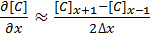
For a grid of points or nodes over a simulation space, each point in the space can describe a number of factors relating to the simulation – concentration, electric field, temperature, and so on. In terms of concentration, the material balance gradients are approximated to the differences in the concentrations of surrounding points. Consider the concentration gradient of species C at point x in one dimension, where [C]x describes the concentration of C at x:
 [1]
[1]
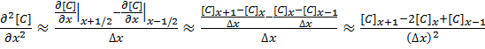
The second derivative around point x is determined by combining the half-differences from the adjacent half-points next to x:
 [2]
[2]
Equations [1] and [2] can be applied to the partial differential equation [3] below to reveal a set of linear equations which can be solved.
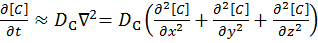
Fick’s first law for the rate of diffusional mass transport can be applied in three dimensions:
 [3]
[3]
where D is the diffusion coefficient of the chemical species, and t is the time. For the dimensional analyses used in this work, the Laplacian is split over the Cartesian dimensions x, y and z.
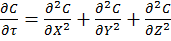
Dimension transformations are often employed to these simulations to relieve the simulation against scaling factors. The expansion of equation [3] given specific dimension transforms not mentioned here give equation [4] to be solved.
 [4]
[4]
The expansion of equation [4] using coefficient collation and expansion by finite differences mentioned in equations [1] and [2] lead to equation [5]:

 [5]
[5]
Equation [5] represents a series of concentrations that can be calculated independently from each other – each concentration can now be solved for each timestep (t) by an explicit algorithm for t+1 from t.
The explicit algorithm is uncommonly used in electrochemical simulation, often due to stability constraints and time taken to simulate. However, it offers complete parallelisation and low thread density – ideal for multi-processor systems and graphics cards – such that these issues should be overcome.
The explicit algorithm is stable when, for equation [4], the Courant–Friedrichs–Lewy condition [6] holds.
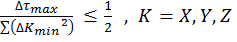 [6]
[6]
Thus the upper bound on the time step is fixed given the minimum grid spacing used.
There are variations of the explicit algorithm to improve this stability, such as the Dufort-Frankel method of considering the concentration at each point as the linear function of time, such that:
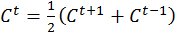 [7]
[7]
However, this method requires knowledge of the concentrations of two steps before the current step, therefore doubling memory usage.
Application to this Review
For the purposes of this review, we generate an x-by-x / x-by-x-by-x grid of points with a relative concentration of 1, where the boundaries are fixed at a relative concentration of 0. The grid is a regular grid, simplifying calculations. As each node in the grid is independently calculable from each other, it would be ideal to spawn as many threads as there are nodes. However, each node has to load the data of the nodes of the previous time step around it, thus we restrict parallelization in one dimension and use an iterative loop to restrict memory loading and increase simulation throughput.
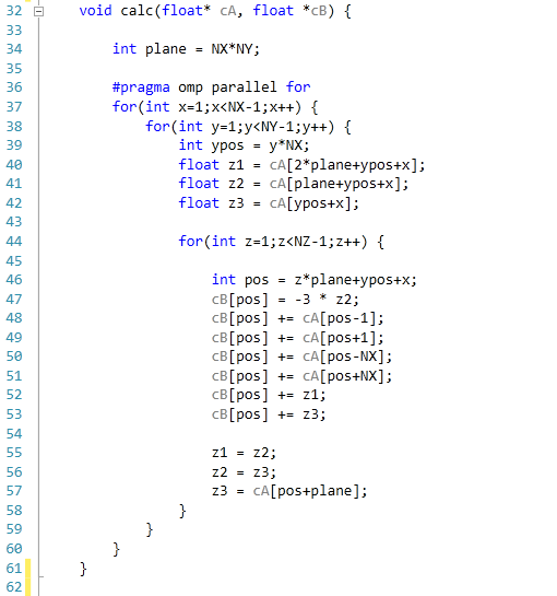
The code was written in Visual Studio C++ 2012 with OpenMP as the multithreaded source. The main functions to do the calculations are as follows.
For 2D:
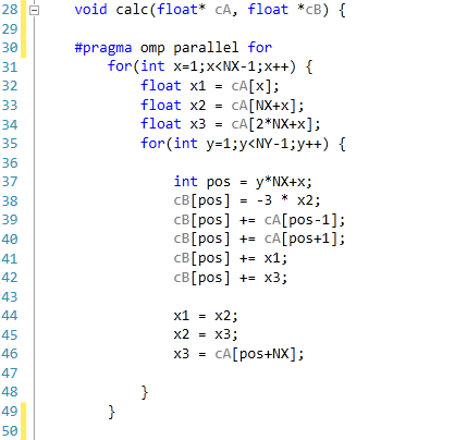
For 3D:
For our scores, we increase the size of the grid from a 2x2 or 2x2x2 until we hit 2GB memory usage. At each stage, the time taken to repeatedly process the grid over many time steps is calculated in terms of ‘million nodes per second’, and the peak value is used for our results.
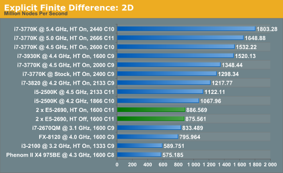
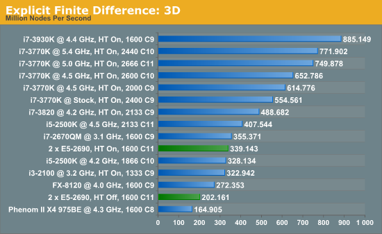
Firstly, the results for our 2D and 3D Explicit Finite Difference simulations are shocking. In 3D, the dual processor system gets beaten by a mobile i7-2670QM (!). In both 2D and 3D, it seems being able to quickly access main memory and L3 caches is top priority. Each processor in the DP machine has to go out to memory when they need a value not in cache, whereas in a single processor machine it can access the L3 cache if the simulation fits wholly in there and the processor can predict which numbers are required next.
Also it should be noted that enabling HyperThreading in 3D gave a better than 50% increase in throughput on the dual processor machine.


64 Comments
View All Comments
toyotabedzrock - Saturday, January 5, 2013 - link
There is a large number of very smart people on Google+. You really should come join us.JlHADJOE - Tuesday, January 8, 2013 - link
Of course there are lots of smart people on G+! You're all google employees right? =PActivate: AMD - Saturday, January 5, 2013 - link
As a fellow chemist, I must say that you have to be some kind of nut to want to do computational/physical chemistry. If you need me, I'll be at the bench!Good article too!
engrpiman - Saturday, January 5, 2013 - link
I didn't read the article in full but what I did read was top notch. I found your simulations and mathematics very interesting. I took a Physics class which was focused in writing code to run mathematical simulations . Using the given java lib. I wrote my own code to calculate PI. When I returned from the gym the program had calculated 3.1 . I then re-wrote the program from scratch and ditched the built in libs. and reran. I had 20 decimals in 30 sec it was an epic improvement.All in all I think your article could be very useful to me.
Thanks for writing.
SodaAnt - Saturday, January 5, 2013 - link
THIS is why I read Anandtech. I'll admit that I wasn't quite in the mood to read all the equations (I'll have to do that later), but really, these kind of reviews make my day.Cardio - Saturday, January 5, 2013 - link
Wonderful review...as always. ThanksHakon - Saturday, January 5, 2013 - link
Hi Ian. Thanks for the nice article. I have one suggestion regarding the explicit finite difference code:You could try to reorder the loops such that the memory access is more cache friendly. Right now 'pos' is incremented by NX (or even NX*NY in 3D) which will generate a lot cache misses for large grids. If you switch the x and the y loop (in the 2D case) this can be avoided.
IanCutress - Saturday, January 5, 2013 - link
Either way I order the loops, each point has to read one up, one down, one left and one right. My current code tries to keep three as consecutive reads and jump once, keeping the old jump in local memory. If I adjusted the loops, I could keep the one dimension in local memory, but I'd have to jump outside twice (both likely cache misses) to get the other data. I couldn't cache those two values as I never use them again in the loop iteration.When I did this code on the GPU, one method was to load an XY block into memory and iterate in the Z-dimension, meaning that each thread per loop iteration only loaded one element, with a few of them loading another for the halo, but all cache aligned.
I hope that makes sense :)
Ian
Hakon - Saturday, January 5, 2013 - link
Yes, but when you access the array 'cA' at 'pos' the CPU will fetch the entire cache line (64 byte in case of your machine, i.e. 16 floats) of the corresponding memory address into the CPU cache. That means that subsequent accesses to say 'pos + 1', 'pos + 2' and so on will be served by the cache. Accessing an array in such a sequential manner is therefore fast.However, when you access an array in a nasty way, e.g. 'NX + x' -> '2*NX + x', -> '3*NX + x', then each such access implies a trip to main memory if NX happens to be large.
That you need to move up / down and sideways in memory does not matter. When you write down the accesses of the code with the reordered loops you will notice that they just access three "lines" in memory in a cache friendly way.
Not reusing the old values of the last iteration should not affect performance in a measurable way. Even if the compiler fails to see this optimization, the accesses will be served by the L1 cache.
Btw, did you allocate the array having NUMA in mind, i.e. did you initialize your memory in an OpenMP loop with the same access pattern as used in the algorithms? I am a bit surprised by the bad performance of your dual Xeon system.
IanCutress - Saturday, January 5, 2013 - link
Memory was allocated via the new command as it is 1D. When using a 2D array the program was much slower. I was unaware you could allocate memory in an OpenMP way, which thinking about it could make the 2D array quicker. I also tried writing the code using the PPL and lambdas, but that was also slower than a simple OpenMP loop.I'm coming at these algorithms from the point of view of a non-CompSci interested in hardware, and the others in the research group were chemists content to write single threaded code on multi-core machines. Transferring the OpenMP variations of that code from a 1P to a 2P, as the results show, give variable results depending on the algorithm.
There are always ways to improve the efficiency of the code (and many ways to make it unreadable), but for a large part moving to the 2P system all depends on how your code performs. Please understand that my examples being within my limits of knowledge and representative of the research I did :) I know that SSE2/SSE4/AVX would probably help, but I have never looked into those. More often than not, these environments are all about research throughput, so rather than spend a few week to improve efficiency by 10% (or less), they'd rather spend that money getting a faster system which theoretically increases the same code throughput 100%.
I'll have a look at switching the loops if I write an article similar to this in the future :)
Ian