Gigabyte GA-7PESH1 Review: A Dual Processor Motherboard through a Scientist’s Eyes
by Ian Cutress on January 5, 2013 10:00 AM EST- Posted in
- Motherboards
- Gigabyte
- C602
Explicit Finite Difference
For a grid of points or nodes over a simulation space, each point in the space can describe a number of factors relating to the simulation – concentration, electric field, temperature, and so on. In terms of concentration, the material balance gradients are approximated to the differences in the concentrations of surrounding points. Consider the concentration gradient of species C at point x in one dimension, where [C]x describes the concentration of C at x:
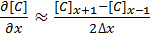 [1]
[1]
The second derivative around point x is determined by combining the half-differences from the adjacent half-points next to x:
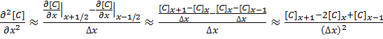 [2]
[2]
Equations [1] and [2] can be applied to the partial differential equation [3] below to reveal a set of linear equations which can be solved.
Fick’s first law for the rate of diffusional mass transport can be applied in three dimensions:
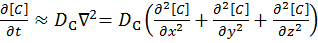 [3]
[3]
where D is the diffusion coefficient of the chemical species, and t is the time. For the dimensional analyses used in this work, the Laplacian is split over the Cartesian dimensions x, y and z.
Dimension transformations are often employed to these simulations to relieve the simulation against scaling factors. The expansion of equation [3] given specific dimension transforms not mentioned here give equation [4] to be solved.
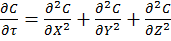 [4]
[4]
The expansion of equation [4] using coefficient collation and expansion by finite differences mentioned in equations [1] and [2] lead to equation [5]:

 [5]
[5]
Equation [5] represents a series of concentrations that can be calculated independently from each other – each concentration can now be solved for each timestep (t) by an explicit algorithm for t+1 from t.
The explicit algorithm is uncommonly used in electrochemical simulation, often due to stability constraints and time taken to simulate. However, it offers complete parallelisation and low thread density – ideal for multi-processor systems and graphics cards – such that these issues should be overcome.
The explicit algorithm is stable when, for equation [4], the Courant–Friedrichs–Lewy condition [6] holds.
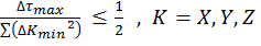 [6]
[6]
Thus the upper bound on the time step is fixed given the minimum grid spacing used.
There are variations of the explicit algorithm to improve this stability, such as the Dufort-Frankel method of considering the concentration at each point as the linear function of time, such that:
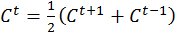 [7]
[7]
However, this method requires knowledge of the concentrations of two steps before the current step, therefore doubling memory usage.
Application to this Review
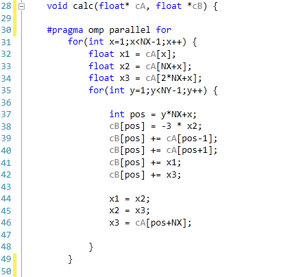
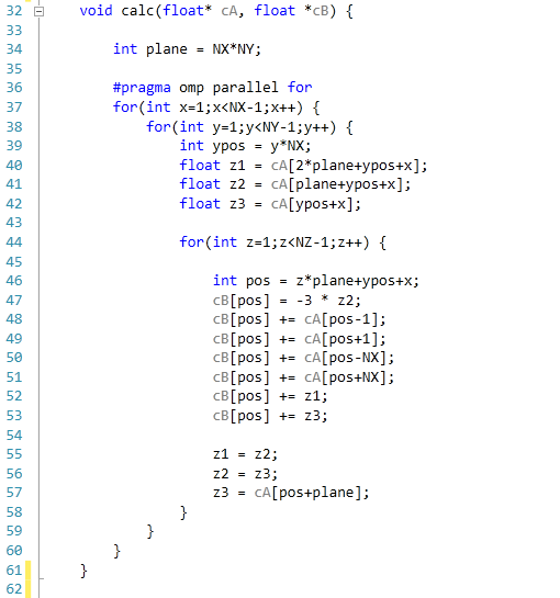
For the purposes of this review, we generate an x-by-x / x-by-x-by-x grid of points with a relative concentration of 1, where the boundaries are fixed at a relative concentration of 0. The grid is a regular grid, simplifying calculations. As each node in the grid is independently calculable from each other, it would be ideal to spawn as many threads as there are nodes. However, each node has to load the data of the nodes of the previous time step around it, thus we restrict parallelization in one dimension and use an iterative loop to restrict memory loading and increase simulation throughput.
The code was written in Visual Studio C++ 2012 with OpenMP as the multithreaded source. The main functions to do the calculations are as follows.
For 2D:
For 3D:
For our scores, we increase the size of the grid from a 2x2 or 2x2x2 until we hit 2GB memory usage. At each stage, the time taken to repeatedly process the grid over many time steps is calculated in terms of ‘million nodes per second’, and the peak value is used for our results.
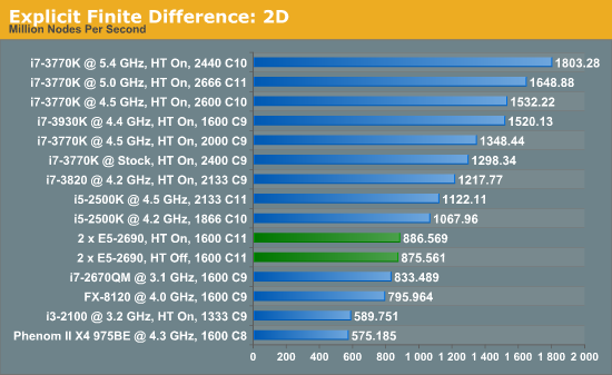
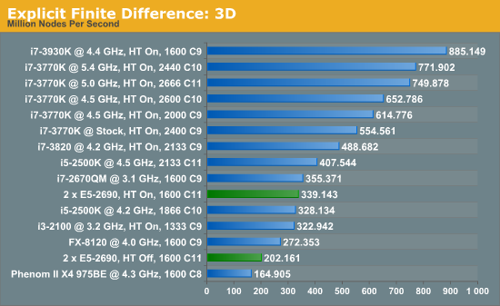
Firstly, the results for our 2D and 3D Explicit Finite Difference simulations are shocking. In 3D, the dual processor system gets beaten by a mobile i7-2670QM (!). In both 2D and 3D, it seems being able to quickly access main memory and L3 caches is top priority. Each processor in the DP machine has to go out to memory when they need a value not in cache, whereas in a single processor machine it can access the L3 cache if the simulation fits wholly in there and the processor can predict which numbers are required next.
Also it should be noted that enabling HyperThreading in 3D gave a better than 50% increase in throughput on the dual processor machine.


64 Comments
View All Comments
mayankleoboy1 - Saturday, January 5, 2013 - link
Ian :How much difference do you think Xeon Phi will make in these very different type of Computations?
Will buying a Xeon Phi "pay itself out" as you said in the above comments ? (or is xeon phi linux only ?)
IanCutress - Saturday, January 5, 2013 - link
As far as we know, Xeon Phi will be released for Linux only to begin with. I have friends who have been able to play with them so far, and getting 700 GFlops+ in DGEMM in double precision.It always comes down to the algorithm with these codes. It seems that if you have single precision code that doesn't mind being in a 2P system, then the GPU route may be preferable. If not, then Phi is an option. I'm hoping to get my hands on one inside H1 this year. I just have to get my hands dirty with Linux as well.
In terms of the codes used here, if I were to guess, the Implicit Finite Difference would probably benefit a lot from Xeon Phi if it works the way I hope it does.
Ian
mayankleoboy1 - Saturday, January 5, 2013 - link
Rather stupid question, but have you tried using PGO builds ?Also, do you build the code with the default optimizations, or use the MSVC equivalent switch of -O2 ?
IanCutress - Saturday, January 5, 2013 - link
Using Visual Studio 2012, all the speed optimisations were enabled including /GL, /O2, /Ot and /fp:fast. For each part I analysed the sections which took the most time using the Performance Analysis tools, and tried to avoid the long memory reads. Hence the Ex-FD uses an iterative loading which actually boosts speed by a good 20-30% than without it.Ian
Klimax - Sunday, January 6, 2013 - link
Interesting. Why not Ox (all optimisations on)BTW: Do you have access to VTune?
IanCutress - Wednesday, January 9, 2013 - link
In case /Ox performs an optimisation for memory over speed in an attempt to balance optimisations. As speed is priority #1, it made more sense to me to optimise for that only. If VS2012 gave more options, I'd adjust accordingly.Never heard of VTune, but I did use the Performance Analysis tools in VS2012 to optimise certain parts of the code.
Ian
Beenthere - Saturday, January 5, 2013 - link
Business and mobo makers do not use 2P mobos to get high benches or performance bragging rights per se. These systems are build for bullet-proof reliability and up time. It does no good for a mobo/system to be 3% faster if it crashes while running a month long analysis. These 2P mobos are about 100% reliability, something rarely found in a enthusiasts mobo.Enterprise mobos are rarely sold by enthusiast marketeers. Newegg has a few enterprise mobos listed primarily because they have started a Newegg Biz website to expand their revenue streams. They don't have much in the line of true enterprise hardware however. It's a token offering because manufacturers are not likely to support whoring of the enterprise market lest they lose all of their quality vendors who provide customer technical product support.
psyq321 - Sunday, January 6, 2013 - link
Actually, ASUS Z9PE-D8 WS allows for some overclocking capabilities.CPU overclocking with 2P/4P Xeon E5 (2600/4600 sequence) is a no-go because Intel explicitly did not store proper ICC data so it is impossible to manipulate BCLK meaningfully (set the different ratios). Oh, and the multipliers are locked :)
However, Z9PE D8 WS allows memory overclocking - I managed to run 100% 24/7 stable with the Samsung ECC 1600 DDR3 "low voltage" RAM (16 GB sticks) - just switching memory voltage from 1.35v to 1.55v allows overclocking memory from 1600 MHz to 2133 MHz.
Why would anyone want to do that in a scientific or b2b environment? The only usage I can see are applications where memory I/O is the biggest bottleneck. Large-scale neural simulations are one of such applications, and getting 10 GB/s more of memory I/O can help a lot - especially if stable.
Also, low-latency trading applications are known to benefit from overclocked hardware and it is, in fact, used in production environment.
Modern hardware does tend to have larger headrooms between the manufacturer's operating point and the limits - if the benefit from an overclock is more benefitial than work invested to find the point where the results become unstable - and, of course, shorter life span of the hardware - then, it can be used. And it is used, for example in some trading scenarios.
Drazick - Saturday, January 5, 2013 - link
Will You, Please, Update Your Google+ Page?It would be much easier to follow you there.
Ryan Smith - Saturday, January 5, 2013 - link
Our Google+ page is just a token page. If you wish to follow us then your best option is to follow our RSS feeds.